Matching

We’ll start with Matching as a potential solution to the fundamental problem of causal inference given an observational dataset.

A crude way to describe matching would be that for each treatment or control subject, we want to find their twin. Imagine if we did have twins that were alike in every possible way and one received the treatment while the other did not. Then, we wouldn’t need randomization! The treatment and control groups are exactly alike EXCEPT that one received treatment and the other did not.

But it’s impossible to find exact twins that are alike in every possible way. In what ways do the twins need to be similar? They need to be similar on variables that we call “confounders”. The formal definition for a confounder is that it’s a variable that is correlated with both the treatment assignment and the outcome.

• “Correlated with treatment assignment” means that the non-randomness of treatment assignment can be partially explained by this variable. If we want to evaluate the impact of smoking on lung cancer, age, gender and ethnicities would be correlated with whether an individual smokes.

• “Correlated with outcome” means that the the variable is also related to the outcome variable.

• Age, gender, and ethnicity might each be confounders since it’s correlated with both the treatment assignment AND the outcome variable.

Typically, it’s impossible to prove that you have measured all the confounders and it’s one of the strongest assumptions we have to make in causal inference. It’s also one of the assumptions that requires subject matter experties and deep thinking about the research question.

But for now, let’s suppose that we DO have all of the confounders. Then, for each treatment subject, we can identify a control subject who are the most similar with respect to confounders.

Fake Data

Let’s generate a fake dataset where treatment is not randomly assigned.
We generate data below such that observations with high values of x1 and x2 are more likely to be assigned treatment.

Let the true treatment effect equal 3.

Since x1 and x2 are correlated with T and y by design, these are our confounder variables. In fact, since there are no other inputs to generate T and y, x1 and x2 are the ONLY two confounders.

import pandas as pd
import numpy as np
np.random.seed(0)
from scipy.special import expit
import seaborn as sns
sns.set(rc={'figure.figsize':(11.7,8.27)})

df = pd.DataFrame({
    "x1": np.random.normal(3,1.5,500),
    "x2": np.random.normal(0,1,500)
})

df["T"] = np.random.binomial(1, expit(df["x1"]+df["x2"]))
df["y1"] = np.array(df[["x1","x2"]]) @ [2,2] + 3
df["y0"] = np.array(df[["x1","x2"]]) @ [2,2]

df["y_obs"] = np.where(df["T"]==1, df["y1"], df["y0"])

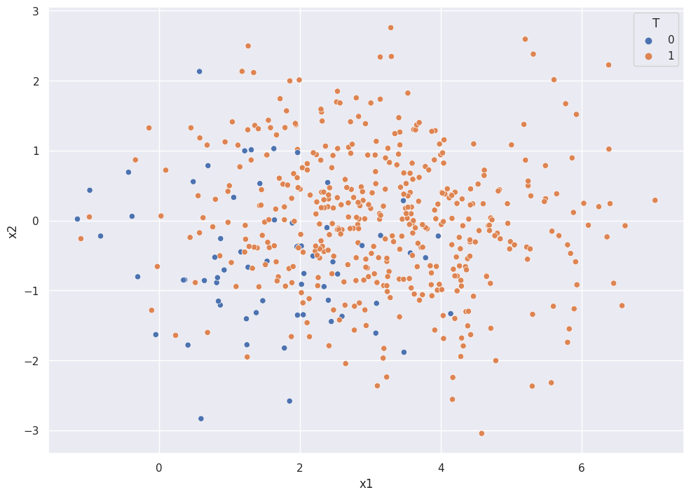
sns.scatterplot(x="x1", y="x2", hue="T", data=df)

<Axes: xlabel='x1', ylabel='x2'>

df["T"].value_counts()

1    436
0     64
Name: T, dtype: int64

The orange points represent the treatment group and the blue points represent the control group.

Without matching, we can simply compute the difference between the averaged observed outcome of the treatment group vs the control group. We call this the “naive” estimate.

dft = df.loc[df["T"]==1].reset_index(drop=True)
dfc = df.loc[df["T"]==0].reset_index(drop=True)
print(f"""The naive estimate of treatment effect is: {dft["y_obs"].mean() - dfc["y_obs"].mean()}""")

The naive estimate of treatment effect is: 7.390547067554589

With matching, we want to match each treatment subject to a control subject on the confounders, x1 and x2.

Notice that there are no control samples with x1>4. Aside from the one point, all observations with x1 > 4 are orange! We call the range of X where both treatment and control observations exist the overlap. Importantly, we CANNOT make causal inference of data in regions with no overlap!

cols = ["x1","x2"]
dist_mat = pd.DataFrame(np.vstack([
    np.linalg.norm(row - dfc[cols], axis=1)
    for row in dft[cols].values
]))

dist_mat = dist_mat[np.min(dist_mat,axis=1) < 0.1].copy()
matches = dist_mat.idxmin(axis=1)
dfc = dfc.loc[dfc.index.isin(matches)].reset_index(drop=True)
dft = dft.loc[dft.index.isin(matches.index)].reset_index(drop=True)

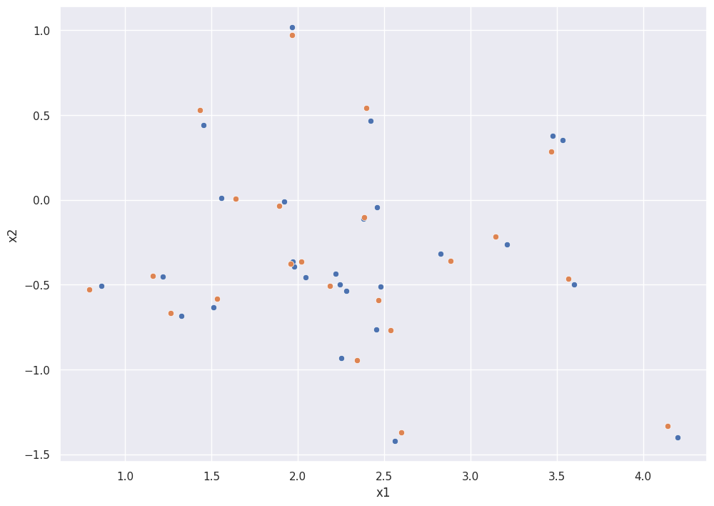
The scatterplot below shows the scatterplot of treatment and control AFTER matching.

Notice that the sample has been restricted to regions where there is overlap.

sns.scatterplot(x="x1", y="x2", data=dft)
sns.scatterplot(x="x1", y="x2", data=dfc)

<Axes: xlabel='x1', ylabel='x2'>

After matching, the estimated treatment effect is much closer to the true value of 3.

print(f"""The matching estimate of treatment effect is: {dft["y_obs"].mean() - dfc["y_obs"].mean()}""")

The matching estimate of treatment effect is: 3.118864451168118