Propensity Scores#
In the matching section, we identified treatment and control subjects that are similar on confounders to construct twin-like pairs.
The critical assumption was that we know the confounders and we’ve measured the confounders.
One problem with matching arises when you have many confounders (or even just 4+). With an increasing number of dimensions, it gets increasingly difficult to identify a match (curse of dimensionality). As an example, if Age and Gender are the only two confounders, then for a 43 year old, male treated subject, it should be easy to find a 43 year old, male control subject. But if you have, Age, Gender, Ethnicity, Zip Code, College-Educated, and Occupation = Dentist, then it might be much more difficult to identify a match.
Propensity scores give you a way to reduce the multiple confounders to a single score. Then, the condition of ignorability will still hold, even if conditioned on this single score alone!
For discussions on proving this property of propensity scores, see here if interested: It only requires basic probability concepts. The intuition is that if two subjects have the same propensity score, they might not be similar on the confounders, but they are similar on average on the confounders.
The basic idea is to define propensity score as the probability of treatment assignment, given confounders: \(\text{score} = P(T=1|X)\). Then, assuming you have all the confounders:
is equivalent to:
Regression Comparison#
How is this differnt from ordinary regression controlling for confounders? This approach handles problems with balance and overlap. Balance means there are equivalent counts of treatment and control subjects. Overlap means that in some region of confounders, both treated and control subjects exist.
If you don’t have balanced data, your estimates may be biased IF your model is incorrectly specified. In the coded example below, I purposefully include a squared term to demonstrate this problem. If your data are balanced, your estimates will still be unbiased even if model is not correctly specified.
If you don’t have overlap, your estimates may be biased if your treatment effect is not constant. If treatment effect is the same for everyone, you can extrapolate results where overlap exists to subjects where there is no overlap.
Algorithm#
Use a (binary) classification model with X as input and T as output.
Predict scores using the model for each subject (these are our propensity scores)
For each treated subject, match the control subject with closest propensity score
For each confounder, plot its distribution for treated and control group using the matched data. There should be strong balance and overlap. If not, you may return to step 1 and try a different model.
Finally, estimate treatment effect using matched data, e.g. regression model with treatment and confounders as covariates.
We want a model in step 1 that is good at predictions. Overfitting is good here and lots of potential for ML tools. Most common model is logistic regression.
Example#
Though we discussed multiple dimensions as one motivation for using propensity scores, we’ll use just two for demonstration simplicity (age, grade)
X = confounders
score = treatment_score
T = treatment
y = outcome
True treatment effect is 10
# Fake Data
import pandas as pd
import numpy as np
from scipy.special import expit
import matplotlib.pyplot as plt
import seaborn as sns
np.random.seed(1)
import statsmodels.api as sm
import patsy

X = pd.DataFrame({
    "age":np.random.normal(40,2,2000),
    "grade":np.random.uniform(70,100,2000),
})
X["grade2"] = X["grade"]**2

df = X.copy()
score = expit(X @ [-2.2,0.84,0.004])
df["T"] = np.random.binomial(1, score)

df["y0"] = X @ [-0.3, 0.4, 0.01] + np.random.normal(0,1,2000)
df["y1"] = X @ [-0.3, 0.4, 0.01] + np.random.normal(0,1,2000) + np.random.normal(10,1,2000)
df["y"] = df["y1"] * df["T"] + df["y0"] * (1 - df["T"])
df["T"].value_counts()
1    1524
0     476
Name: T, dtype: int64
df.head()
| age | grade | grade2 | T | y0 | y1 | y | |
|---|---|---|---|---|---|---|---|
| 0 | 43.248691 | 96.375957 | 9288.325052 | 1 | 119.300572 | 125.185285 | 125.185285 |
| 1 | 38.776487 | 75.064006 | 5634.604952 | 1 | 75.253192 | 87.427215 | 87.427215 |
| 2 | 38.943656 | 91.106432 | 8300.381946 | 1 | 108.770679 | 116.934327 | 116.934327 |
| 3 | 37.854063 | 97.517805 | 9509.722248 | 1 | 122.086311 | 131.058887 | 131.058887 |
| 4 | 41.730815 | 74.522190 | 5553.556769 | 0 | 71.268553 | 83.779786 | 71.268553 |
Naive Estimate#
Since model is incorrectly specified, our estimate is biased
f = 'y ~ age + grade + T'
_T, _X = patsy.dmatrices(f, df, return_type='dataframe')
naiveMod = sm.OLS(_T, _X)
resnaive = naiveMod.fit()
print(resnaive.summary())
                            OLS Regression Results
==============================================================================
Dep. Variable:                      y   R-squared:                       0.995
Model:                            OLS   Adj. R-squared:                  0.995
Method:                 Least Squares   F-statistic:                 1.471e+05
Date:                Thu, 01 Jun 2023   Prob (F-statistic):               0.00
Time:                        12:45:32   Log-Likelihood:                -3554.7
No. Observations:                2000   AIC:                             7117.
Df Residuals:                    1996   BIC:                             7140.
Df Model:                           3
Covariance Type:            nonrobust
==============================================================================
                 coef    std err          t      P>|t|      [0.025      0.975]
------------------------------------------------------------------------------
Intercept    -69.9842      0.705    -99.204      0.000     -71.368     -68.601
age           -0.3803      0.017    -22.245      0.000      -0.414      -0.347
grade          2.1299      0.005    411.571      0.000       2.120       2.140
T              8.9722      0.109     82.295      0.000       8.758       9.186
==============================================================================
Omnibus:                        0.656   Durbin-Watson:                   2.040
Prob(Omnibus):                  0.720   Jarque-Bera (JB):                0.721
Skew:                           0.022   Prob(JB):                        0.697
Kurtosis:                       2.918   Cond. No.                     2.07e+03
==============================================================================

Notes:
[1] Standard Errors assume that the covariance matrix of the errors is correctly specified.
[2] The condition number is large, 2.07e+03. This might indicate that there are
strong multicollinearity or other numerical problems.
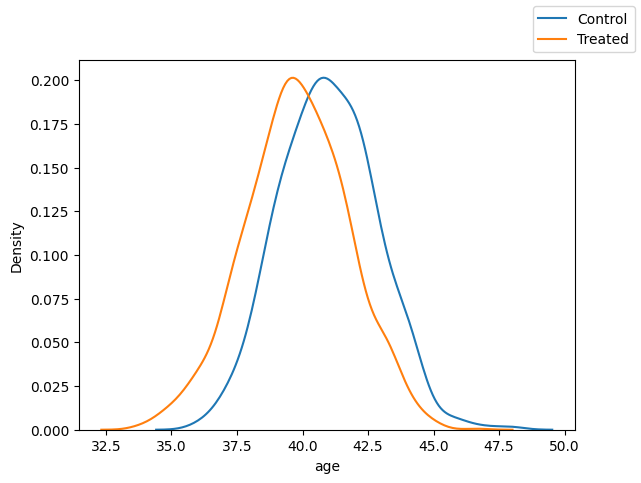
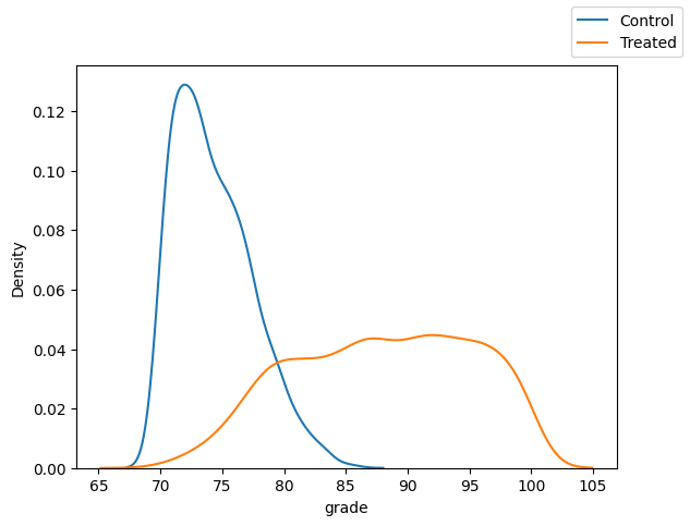
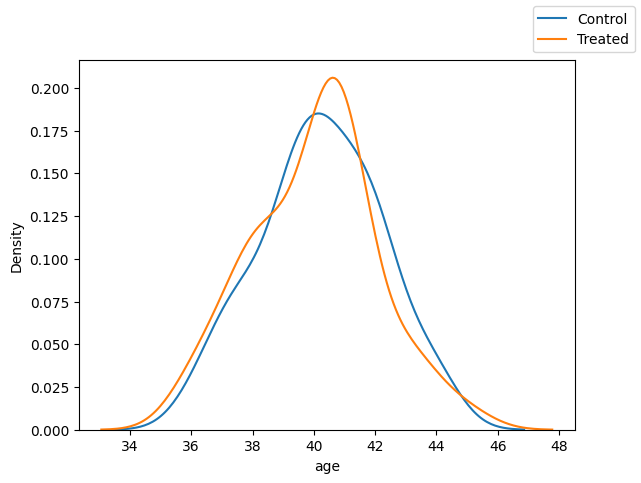
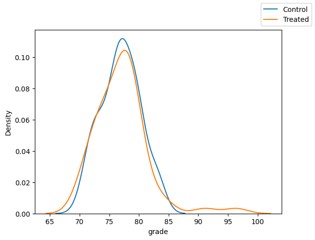
Note the imbalanced and lack of overlap between treatment and control groups.
It’s not so bad for age, but problematic with grade.
var = "age"
fig, ax = plt.subplots(1, 1)
sns.kdeplot(x=var, data=df.loc[df["T"]==0])
sns.kdeplot(x=var, data=df.loc[df["T"]==1])
fig.legend(labels=["Control", "Treated"])
<matplotlib.legend.Legend at 0x7fbd0a6262b0>
var = "grade"
fig, ax = plt.subplots(1, 1)
sns.kdeplot(x=var, data=df.loc[df["T"]==0])
sns.kdeplot(x=var, data=df.loc[df["T"]==1])
fig.legend(labels=["Control", "Treated"])
<matplotlib.legend.Legend at 0x7fbd0a1fdaf0>
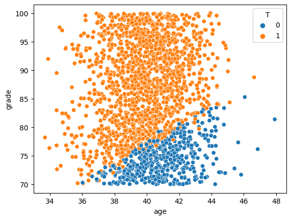
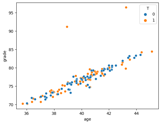
# looking at joint distribution, shows extent of overlap issue
sns.scatterplot(x='age', y='grade', hue="T", data=df)
<Axes: xlabel='age', ylabel='grade'>
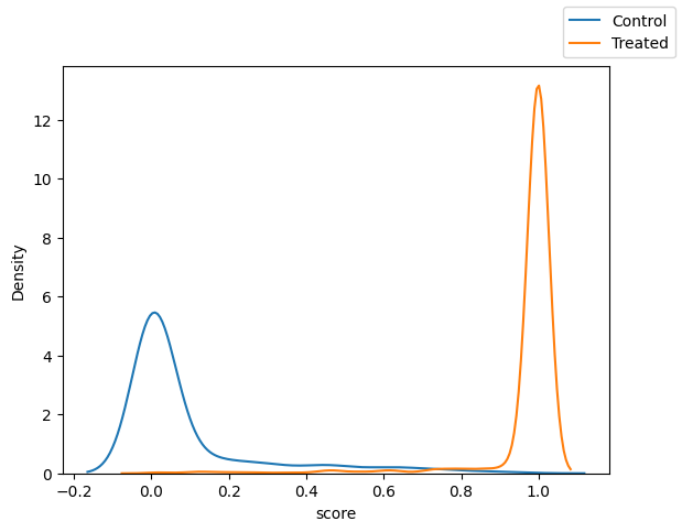
Fit logistic regression to predict scores#
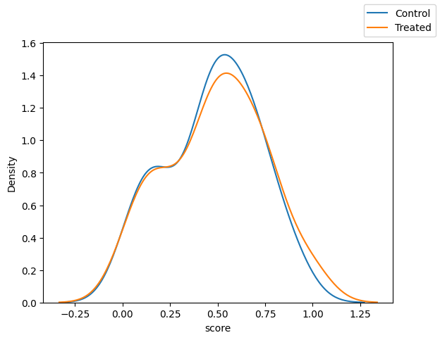
Notice the imbalance in scores prior to matching.
f = 'T ~ age + grade + age*grade'
_T, _X = patsy.dmatrices(f, df, return_type='dataframe')
mod = sm.GLM(_T, _X, family=sm.families.Binomial())
res = mod.fit()
df["score"] = res.predict()

fig, ax = plt.subplots(1, 1)
sns.kdeplot(x="score",data=df.loc[df["T"]==0])
sns.kdeplot(x="score",data=df.loc[df["T"]==1])
fig.legend(labels=["Control", "Treated"])
<matplotlib.legend.Legend at 0x7fbd9824e310>
Match:#
dft = df.loc[df["T"]==1].reset_index(drop=True)
dfc = df.loc[df["T"]==0].reset_index(drop=True)
cands = dfc["score"]
matched_list = {"c":[],"t":[]}
for idx,score in dft["score"].items():
    dist = abs(cands-score)
    if min(dist) < 0.1:
        matched = dist.idxmin()
        matched_list["t"].append(idx)
        matched_list["c"].append(matched)
        cands = cands.drop(matched)
df_matched = pd.concat(
    [
        dft.loc[matched_list["t"]],
        dfc.loc[matched_list["c"]],
    ]
    ,
    axis=0
)
Examine Balance/Overlap of Matched Data#
Scores:
fig, ax = plt.subplots(1, 1)
sns.kdeplot(x="score",data=df_matched.loc[df_matched["T"]==0])
sns.kdeplot(x="score",data=df_matched.loc[df_matched["T"]==1])
fig.legend(labels=["Control", "Treated"])
<matplotlib.legend.Legend at 0x7fbd043a68b0>
Age
fig, ax = plt.subplots(1, 1)
sns.kdeplot(x="age",data=df_matched.loc[df_matched["T"]==0])
sns.kdeplot(x="age",data=df_matched.loc[df_matched["T"]==1])
fig.legend(labels=["Control", "Treated"])
<matplotlib.legend.Legend at 0x7fbd04324730>
Grade
fig, ax = plt.subplots(1, 1)
sns.kdeplot(x="grade",data=df_matched.loc[df_matched["T"]==0])
sns.kdeplot(x="grade",data=df_matched.loc[df_matched["T"]==1])
fig.legend(labels=["Control", "Treated"])
<matplotlib.legend.Legend at 0x7fbd05d87340>
Age AND Grade
sns.scatterplot(x='age', y='grade', hue="T", data=df_matched)
<Axes: xlabel='age', ylabel='grade'>
Estimate Treatment Effect:#
Since data are balanced, our estimate is unbiased, even with incorrect model specification.
f = 'y ~ age + grade + T'
_T, _X = patsy.dmatrices(f, df_matched, return_type='dataframe')
mod = sm.OLS(_T, _X)
resOLS = mod.fit()
print(resOLS.summary())
                            OLS Regression Results
==============================================================================
Dep. Variable:                      y   R-squared:                       0.983
Model:                            OLS   Adj. R-squared:                  0.982
Method:                 Least Squares   F-statistic:                     2374.
Date:                Thu, 01 Jun 2023   Prob (F-statistic):          2.58e-109
Time:                        12:45:34   Log-Likelihood:                -200.23
No. Observations:                 128   AIC:                             408.5
Df Residuals:                     124   BIC:                             419.9
Df Model:                           3
Covariance Type:            nonrobust
==============================================================================
                 coef    std err          t      P>|t|      [0.025      0.975]
------------------------------------------------------------------------------
Intercept    -56.4142      2.180    -25.873      0.000     -60.730     -52.098
age           -0.4163      0.098     -4.255      0.000      -0.610      -0.223
grade          1.9652      0.050     39.288      0.000       1.866       2.064
T             10.3987      0.209     49.648      0.000       9.984      10.813
==============================================================================
Omnibus:                        1.992   Durbin-Watson:                   2.355
Prob(Omnibus):                  0.369   Jarque-Bera (JB):                1.885
Skew:                           0.209   Prob(JB):                        0.390
Kurtosis:                       2.577   Cond. No.                     1.83e+03
==============================================================================

Notes:
[1] Standard Errors assume that the covariance matrix of the errors is correctly specified.
[2] The condition number is large, 1.83e+03. This might indicate that there are
strong multicollinearity or other numerical problems.