Continuous Distributions#
Uniform
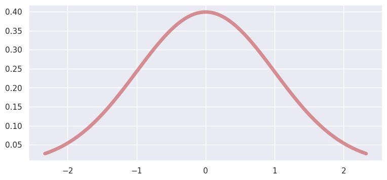
Normal
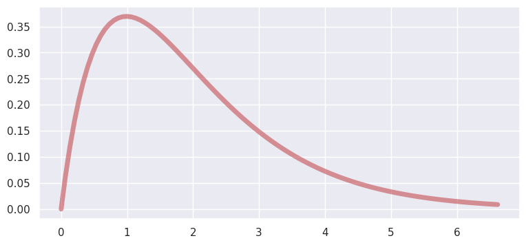
Gamma
Exponential
Chi-Square
Beta
Unlike discrete distributions, real-world examples aren’t as interesting for these distributions. Which is not to say that they don’t exist, but that these distributions are often used differently in applied statistics.
Normal, chi-square, and student’s t- distributions are often used in statistical tests.
All of these distributions frequently come up as prior distributions in Bayesian models.
For our purposes, it’s probably sufficient to be familiar with the shape of the distributions and their domain (e.g. (0,inf), (-inf,inf)).
Good resource for derivation of exponential / gamma/ chi-square
Show code cell content
from IPython import get_ipython
if get_ipython() is not None:
    get_ipython().run_line_magic('load_ext', 'autoreload')
    get_ipython().run_line_magic('autoreload', '2')
import seaborn as sns; sns.set()
import matplotlib.pyplot as plt
import numpy as np
import pandas as pd
from scipy import stats
sns.set(rc={'figure.figsize':(9,4)})
Uniform#
PDF:
mean: \(\frac{\theta_1 + \theta_2}{2}\)
var: \(\frac{(\theta_2-\theta_1)^2}{12}\)
domain: \((-\infty, \infty)\)
from scipy.stats import uniform
fig, ax = plt.subplots(1, 1)
x = np.linspace(uniform.ppf(0.01),
                uniform.ppf(0.99), 100)
ax.plot(x, uniform.pdf(x),
       'r-', lw=5, alpha=0.6, label='uniform pdf')
[<matplotlib.lines.Line2D at 0x7f640caf6bb0>]
Normal#
PDF:
mean: \(\mu\)
var: \(\sigma^2\)
domain: \((-\infty, \infty)\)
from scipy.stats import norm
fig, ax = plt.subplots(1, 1)
x = np.linspace(norm.ppf(0.01),
                norm.ppf(0.99), 100)
ax.plot(x, norm.pdf(x),
       'r-', lw=5, alpha=0.6, label='normal pdf')
[<matplotlib.lines.Line2D at 0x7f640cac47f0>]
Gamma#
PDF:
Given \(\alpha>0\) and \(\beta>0\),
Where \(\Gamma(\alpha) = \int_0^\infty y^{\alpha-1}e^{-y} dy\)
mean: \(\alpha\beta\)
var: \(\alpha\beta^2\)
domain: \((0, \infty)\)
# scipy uses gamma with gamma.pdf(x, a, loc, scale) with scale = 1 / beta
# this is equivalent to gamma.pdf(y, a) / scale with y = (x-loc) / scale
from scipy.stats import gamma
fig, ax = plt.subplots(1, 1)
a = 1.99
x = np.linspace(gamma.ppf(0, a),
                gamma.ppf(0.99, a), 100)
ax.plot(x, gamma.pdf(x, a),
       'r-', lw=5, alpha=0.6, label='gamma pdf')
[<matplotlib.lines.Line2D at 0x7f640c9c66a0>]
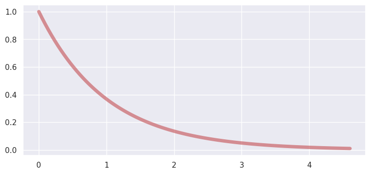
Exponential#
PDF:
mean: \(\beta\)
var: \(\beta^2\)
domain: \((0, \infty)\)
Exponential is a special case of gamma, with parameter \(\alpha=1\) and \(\beta>0\)
from scipy.stats import expon
fig, ax = plt.subplots(1, 1)
x = np.linspace(expon.ppf(0),
                expon.ppf(0.99), 100)
ax.plot(x, expon.pdf(x),
       'r-', lw=5, alpha=0.6, label='exponential pdf')
[<matplotlib.lines.Line2D at 0x7f640c94e1c0>]
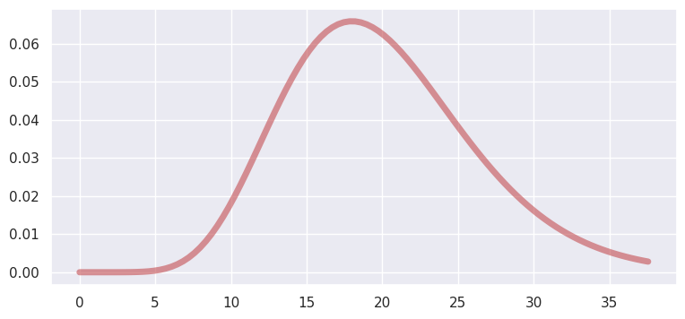
Chi-Square#
PDF:
is said to be a chi-square distribution with v degrees of freedom
mean: \(v\)
var: \(2v\)
domain: \((0, \infty)\)
Chi-Square is a special case of gamma, with parameter \(\alpha=\frac{v}{2}\) and \(\beta=2\)
from scipy.stats import chi2
fig, ax = plt.subplots(1, 1)
df=20
x = np.linspace(chi2.ppf(0, df),
                chi2.ppf(0.99, df), 100)
ax.plot(x, chi2.pdf(x, df),
       'r-', lw=5, alpha=0.6, label='chi square pdf')
[<matplotlib.lines.Line2D at 0x7f640a892f70>]
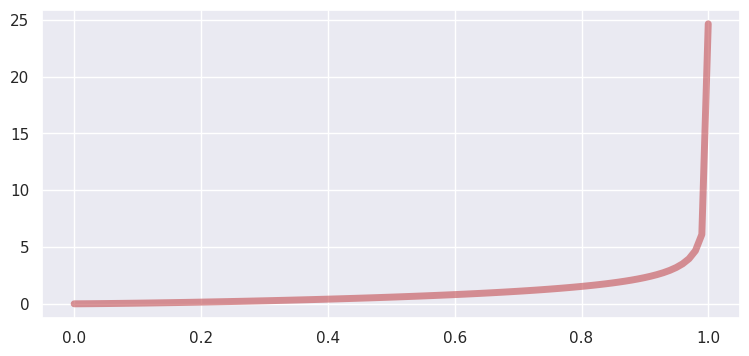
Beta#
PDF:
Given \(\alpha>0\) and \(\beta>0\),
Where \(B(\alpha, \beta) = \int_0^1 y^{\alpha-1}(1-y)^{\beta-1} dy = \frac{\Gamma(\alpha)\Gamma(\beta)}{\Gamma(\alpha+\beta)}\)
mean: \(\frac{\alpha}{\alpha + \beta}\)
var: \(\frac{\alpha\beta}{(\alpha + \beta)^2(\alpha+\beta+1)}\)
domain: \((0, 1)\)
from scipy.stats import beta
fig, ax = plt.subplots(1, 1)
a, b = 2.31, 0.627
x = np.linspace(beta.ppf(0, a, b),
                beta.ppf(0.99, a, b), 100)
ax.plot(x, beta.pdf(x, a, b),
       'r-', lw=5, alpha=0.6, label='chi square pdf')
[<matplotlib.lines.Line2D at 0x7f640a8159d0>]