Shallow Neural Network#
Given two inputs, \(x_1\) and \(x_2\), and an output \(y\), and n = 100, we use a shallow neural network to build a prediction model. The purpose of this notbook is to show how a simple neural network works.
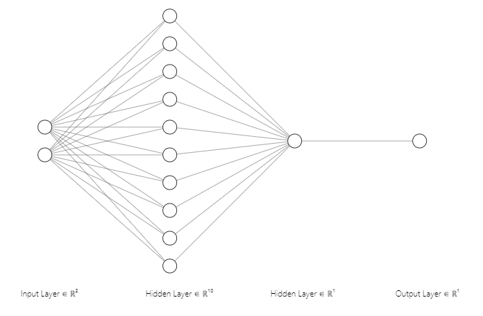
The below diagram illustrates a shallow neural network with an input layer, two hidden layers, and an output layer. The input layer has two nodes, representing the two input vectors, \(x_1\) and \(x_2\). The first hidden layer has 10 nodes, the second hidden layer has 1 node, and the output layer has one node, representing the output vector, \(y\).
import numpy as np
np.random.seed(0)
from tqdm import tqdm
import seaborn as sns
sns.set(rc={'figure.figsize':(11.7,8.27)})

m = 10000
x1 = np.random.normal(0, 2, m)
x2 = np.random.normal(10, 2, m)
X = np.stack([x1, x2])
y = 2*x1 * x2 + 2
Training Overview#
As a brief overview, the idea behind training is (1) to obtain predicted values then (2) use an optimization method (e.g. gradient descent) to improve weights. We iterate this process until convergence or until our we think that the model is doing well.
The prediction step is called forward propagation.
The optimization / weight-improving step is called backward propagation.
Forward Propagation#
“Forward Propagation” means we feed the inputs into the model to get our predicted output values. Since the values of the weights are unknown, we initialize the weights randomly.
We can vectorize operations by using a 2 x 100 \(X\) matrix for inputs (since n = 100 and 2 features) and a 10 x 2 \(W\) matrix (since hidden layer has 10 nodes and inputs from 2 nodes).:
W1 = np.random.rand(10, 2)
X = np.stack([x1, x2])
b1 = np.random.rand(10, 1)
print((W1 @ X).shape)
# b is broadcasted over the 100 samples
print((W1 @ X + b1).shape)
(10, 10000)
(10, 10000)
Z1 = W1 @ X + b1
A1 = np.apply_along_axis(sigmoid, 1, Z1)
print(A1.shape)
(10, 10000)
We repeat for the second hidden layer, which has one node and takes in the output from the previous hidden layer, \(a\) as its own input. So W2 for this layer is 1x10 since it has one node and takes in 10 inputs from previuos layer. And the output of this layer are our 1x100 predictions:
W2 = np.random.rand(1, 10)
b = np.random.rand(1, 1)
Z2 = W2 @ A1 + b
print(Z2.shape)
(1, 10000)
A2 = np.apply_along_axis(sigmoid, 1, Z2)
A2.shape
(1, 10000)
Back Propagation#
First, we need our loss funtion. Here, we’ll use average error, where error is the difference between predicted and actual values.
Loss Function:
Second, we use gradient descent as our optimization algorithm. At each step, we compute the partial derivative of the loss function with respect to each weight. Then we subtract \(\alpha\) times the derivative (where \(\alpha\) is the learning rate) from the weight to get our new weight estimate, e.g.
Summary of Forward Propagation \(Z^{[1]}\) indicates \(Z\) in first hidden layer:
\(Z^{[1]} = W^{[1]}X + b^{[1]}\)
\(A^{[1]} = sigmoid(Z^{[1]})\)
\(Z^{[2]} = W^{[2]}A^{[1]} + b^{[2]}\)
\(A^{[2]} = sigmoid(Z^{[2]})\)
\(\hat{y} = A^{[2]}\)
Back Propagation:
Remember that \(\frac{\partial{J}}{\partial{w2}} = \frac{\partial{J}}{\partial{z2}} \frac{\partial{z2}}{\partial{w2}}\)
\(dZ^{[2]} = A^{[2]} - y\)
\(dW^{[2]} = \frac{1}{m} dZ^{[2]} A^{[1]T}\)
\(db^{[2]} = \frac{1}{m} sum(dZ^{[2]})\)
\(dZ^{[1]} = W^{[2]}dZ^{[2]} * g'^{[1]}(dZ^{[1]})\)
\(dW^{[1]} = \frac{1}{m} dZ^{[1]} X^{T}\)
\(db^{[1]} = \frac{1}{m} sum(dZ^{[1]})\)
dZ2 = A2 - y
dW2 = (1/m) * dZ2 * np.transpose(A2)
db2 = (1/m) * np.sum(dZ2)

# since g(z) is sigmoid,
# g'(z) is g(z) * (1 - g(z))
dZ1 = np.transpose(W2) @ dZ2 * (A1 * (1 - A1))
dW1 = (1/m) * dZ1 @ np.transpose(X)
db = (1/m) * np.sum(Z1)
Putting it Together#
Put together the weight initialization, forward propagation, and backward propagation steps. Also add an updating step, which requires a “learning rate”: the pace at which the model “learns”.
class nn:

    def __init__(self, X, y, alpha, n_iter=100):
        self.X = X
        self.y = y
        self.m = X.shape[1]
        self.alpha = alpha
        self.n_iter = n_iter

    def initialize_weights(self):
        self.W1 = np.random.rand(10, 2)
        self.b1 = np.random.rand(10, 1)
        self.W2 = np.random.rand(1, 10)
        self.b2 = np.random.rand(1, 1)

    def sigmoid(self, x):
        return 1 / (1 + np.exp(-x))

    def forward(self):
        self.Z1 = self.W1 @ self.X + self.b1
        self.A1 = self.sigmoid(self.Z1)
        self.Z2 = self.W2 @ self.A1 + self.b2
        self.A2 = self.Z2

    def backward(self):
        self.dZ2 = self.A2 - self.y
        self.dW2 = (1/self.m) * self.dZ2 @ np.transpose(self.A1)
        self.db2 = (1/self.m) * np.sum(self.dZ2)
        self.dZ1 = np.transpose(self.W2) @ self.dZ2 * (self.A1 * (1 - self.A1))
        self.dW1 = (1/self.m) * self.dZ1 @ np.transpose(self.X)
        self.db1 = (1/self.m) * np.sum(self.dZ1)

    def update(self):
        self.W1 -= self.alpha * self.dW1
        self.W2 -= self.alpha * self.dW2
        self.b1 -= self.alpha * self.db1
        self.b2 -= self.alpha * self.db2

    def __call__(self):

        self.initialize_weights()
        self.loss = []
        for i in range(self.n_iter):
            self.forward()
            self.backward()
            self.update()
            self.loss.append(np.mean(self.A2 - self.y))
        self.forward()

        return self.A2
shallow = nn(X, y, alpha=0.001, n_iter=10_000)
y_pred = shallow()
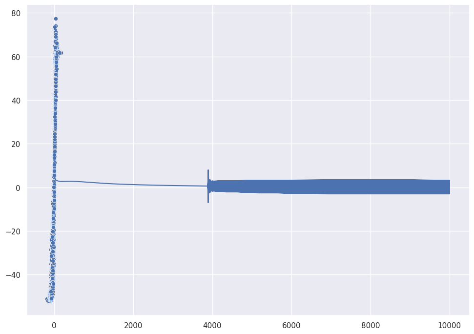
sns.lineplot([i for i in range(shallow.n_iter)], shallow.loss)
sns.scatterplot(y, y_pred[-1,:])
/home/chansoo/projects/statsbook/.venv/lib/python3.8/site-packages/seaborn/_decorators.py:36: FutureWarning: Pass the following variables as keyword args: x, y. From version 0.12, the only valid positional argument will be `data`, and passing other arguments without an explicit keyword will result in an error or misinterpretation.
  warnings.warn(
<Axes: >
Hyperparameters#
In this simple model, the hyperparameters include:
learning rate
# of iterations
# of hidden layers
# of hidden units
choice of activation functions