Demo#
A logitic regression is used when the dependent variable is a binary outcome.
It uses a logit link function to relate the continuous \((-\inf,\inf)\) linear component (\(\eta\)) to the \((0,1)\) dependent variable, \(P(y_i=1)\). Then a bernoulli trial to convert these probabilities into binary data, 0 or 1.
import numpy as np
import pandas as pd
import statsmodels.api as sm
from sklearn.linear_model import LogisticRegression
import seaborn as sns
import patsy
sns.set(rc={'figure.figsize':(11.7,8.27)})
Generate Fake Data#
We generate two independent variables x1 and x2. We let \(\eta\) be the linear component, \(X\beta\), then inverse_logit(\(\eta\)) is the link function that converts \(\eta\) to a probability. (inverse logit = logistic)
Then y is the outcome of a bernoulli trial (binomial with 1 trial) with these probabilities.
def inverse_logit(x):
    return(1 / (1 + np.exp(-x)))

n = 500
np.random.seed(0)
df = pd.DataFrame({
    "x1":np.random.normal(1,1,n),
    "x2":np.random.normal(-2,1,n),
})

df["eta"] = - 3 + 2*df["x1"] - 1.5*df["x2"]
df["probs"] = inverse_logit(df["eta"])
df["y"] = np.random.binomial(size=n, n=1, p=df["probs"])
df["y"].value_counts()
1    370
0    130
Name: y, dtype: int64
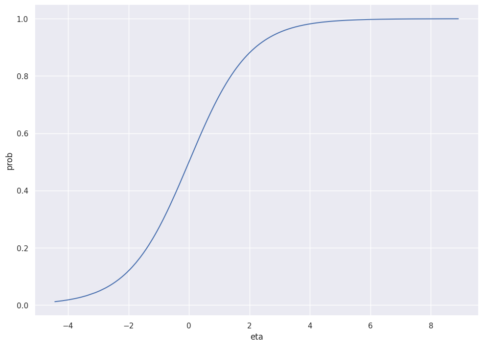
The plot below shows the inverse_logit relation between \(\eta\) and the probs.
g = sns.lineplot(df["eta"], inverse_logit(df["eta"]))
g.set_xlabel("eta")
g.set_ylabel("prob")
/home/chansoo/projects/statsbook/.venv/lib/python3.8/site-packages/seaborn/_decorators.py:36: FutureWarning: Pass the following variables as keyword args: x, y. From version 0.12, the only valid positional argument will be `data`, and passing other arguments without an explicit keyword will result in an error or misinterpretation.
  warnings.warn(
Text(0, 0.5, 'prob')
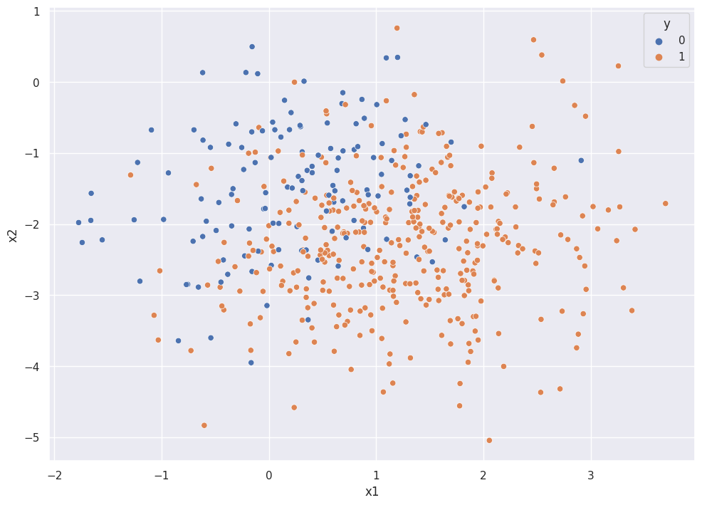
The plot below shows the binary classification problem, with \(y \in [{0,1}]\).
sns.scatterplot(df["x1"], df["x2"], hue=df["y"])
/home/chansoo/projects/statsbook/.venv/lib/python3.8/site-packages/seaborn/_decorators.py:36: FutureWarning: Pass the following variables as keyword args: x, y. From version 0.12, the only valid positional argument will be `data`, and passing other arguments without an explicit keyword will result in an error or misinterpretation.
  warnings.warn(
<Axes: xlabel='x1', ylabel='x2'>
f = 'y ~ x1 + x2'
y, X = patsy.dmatrices(f, df, return_type='dataframe')
Statsmodels#
There are a couple ways to run logistic regression using statsmodels. Note that in both cases, in the model output, the Link function is “logit”.
See the “interpretation” page for more info about interpreting regression results.
mod = sm.Logit(y, X)
res = mod.fit()
print(res.summary())
Optimization terminated successfully.
         Current function value: 0.381869
         Iterations 7
                           Logit Regression Results
==============================================================================
Dep. Variable:                      y   No. Observations:                  500
Model:                          Logit   Df Residuals:                      497
Method:                           MLE   Df Model:                            2
Date:                Thu, 01 Jun 2023   Pseudo R-squ.:                  0.3336
Time:                        12:45:51   Log-Likelihood:                -190.93
converged:                       True   LL-Null:                       -286.53
Covariance Type:            nonrobust   LLR p-value:                 3.048e-42
==============================================================================
                 coef    std err          z      P>|z|      [0.025      0.975]
------------------------------------------------------------------------------
Intercept     -2.2766      0.351     -6.495      0.000      -2.964      -1.590
x1             1.6063      0.179      8.950      0.000       1.255       1.958
x2            -1.1719      0.156     -7.521      0.000      -1.477      -0.866
==============================================================================
# alternatively, using GLM and specifying the Binomial family for logistic regression
mod = sm.GLM(y, X, family=sm.families.Binomial())
res2 = mod.fit()
print(res2.summary())
                 Generalized Linear Model Regression Results
==============================================================================
Dep. Variable:                      y   No. Observations:                  500
Model:                            GLM   Df Residuals:                      497
Model Family:                Binomial   Df Model:                            2
Link Function:                  Logit   Scale:                          1.0000
Method:                          IRLS   Log-Likelihood:                -190.93
Date:                Thu, 01 Jun 2023   Deviance:                       381.87
Time:                        12:45:51   Pearson chi2:                     447.
No. Iterations:                     6   Pseudo R-squ. (CS):             0.3178
Covariance Type:            nonrobust
==============================================================================
                 coef    std err          z      P>|z|      [0.025      0.975]
------------------------------------------------------------------------------
Intercept     -2.2766      0.351     -6.495      0.000      -2.964      -1.590
x1             1.6063      0.179      8.950      0.000       1.255       1.958
x2            -1.1719      0.156     -7.521      0.000      -1.477      -0.866
==============================================================================
sklearn#
model = LogisticRegression(fit_intercept = False)
mdl = model.fit(X, y)
model.coef_
/home/chansoo/projects/statsbook/.venv/lib/python3.8/site-packages/sklearn/utils/validation.py:1143: DataConversionWarning: A column-vector y was passed when a 1d array was expected. Please change the shape of y to (n_samples, ), for example using ravel().
  y = column_or_1d(y, warn=True)
array([[-1.95377627, 1.48859512, -1.04496352]])
default setting is regularization; turn it off by setting penalty='none'
model = LogisticRegression(fit_intercept = False, penalty='none')
mdl = model.fit(X, y)
model.coef_
/home/chansoo/projects/statsbook/.venv/lib/python3.8/site-packages/sklearn/linear_model/_logistic.py:1173: FutureWarning: `penalty='none'`has been deprecated in 1.2 and will be removed in 1.4. To keep the past behaviour, set `penalty=None`.
  warnings.warn(
/home/chansoo/projects/statsbook/.venv/lib/python3.8/site-packages/sklearn/utils/validation.py:1143: DataConversionWarning: A column-vector y was passed when a 1d array was expected. Please change the shape of y to (n_samples, ), for example using ravel().
  y = column_or_1d(y, warn=True)
array([[-2.27659181, 1.60631138, -1.17185961]])