Confidence Intervals

import numpy as np
import pandas as pd
import seaborn as sns
import matplotlib.pyplot as plt
np.random.seed(0)
import scipy.stats as st

Intro

First, we generate a fake population data.
We’ll use a chi square distribution for no particular reason.
It doesn’t have to follow a distribution at all. The plot is shown below.

# Fake Data
population = np.random.chisquare(5,10000)
sns.histplot(population)
true_mean = np.mean(population)
print(true_mean)

4.961307278243971

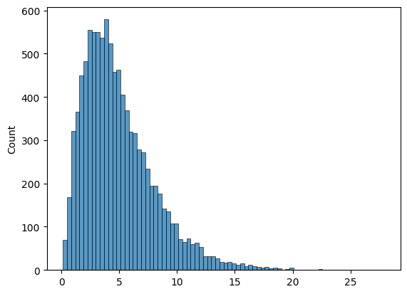
print(f"For this distribution the true mean is {true_mean}")

For this distribution the true mean is 4.961307278243971

The plan is to simulate repeated samples from this population.
For each sample, we compute a lower bound and an upper bound for the confidence interval of a sample mean.

First, let’s declare our inputs. The z-value for a 95% confidence interval is 1.96.

sample_size = 40
zvalue = 1.96

Simulations

Next, we run the simulations:

We initialize a dictionary “intervals” to store the lower and upper bound of our confidence intervals.

We run the simulation for 200 iterations. We can make this value an input too, but hardcoded below for simplicity.

Remember, the bounds of the confidence interval are given by:

\[\pm \ z_{\alpha/2} * \frac{s}{\sqrt{n}}\]

intervals = {
    "low":[],
    "high":[],
}

for i in range(200):
    sample = np.random.choice(population, sample_size)
    sample_mean = np.mean(sample)
    sample_std = np.std(sample)
    intervals["low"].append(sample_mean-zvalue*(sample_std/np.sqrt(sample_size)))
    intervals["high"].append(sample_mean+zvalue*(sample_std/np.sqrt(sample_size)))

We convert the results into a dataframe. And flag the intervals that do not contain the true mean.

df = pd.DataFrame(intervals).reset_index()
df["reject"] = np.where(
    (df["low"]>true_mean) | (df["high"]<true_mean),
    "r",
    "b"
)

Let’s plot results:

sns.set(rc={'figure.figsize':(11.7,8.27)})
sns.scatterplot(df["low"],df["index"], hue = df["reject"])
sns.scatterplot(df["high"],df["index"], hue = df["reject"], legend=False)
ints = plt.xlabel("Intervals")

/home/chansoo/projects/statsbook/.venv/lib/python3.8/site-packages/seaborn/_decorators.py:36: FutureWarning: Pass the following variables as keyword args: x, y. From version 0.12, the only valid positional argument will be `data`, and passing other arguments without an explicit keyword will result in an error or misinterpretation.
  warnings.warn(
/home/chansoo/projects/statsbook/.venv/lib/python3.8/site-packages/seaborn/_decorators.py:36: FutureWarning: Pass the following variables as keyword args: x, y. From version 0.12, the only valid positional argument will be `data`, and passing other arguments without an explicit keyword will result in an error or misinterpretation.
  warnings.warn(

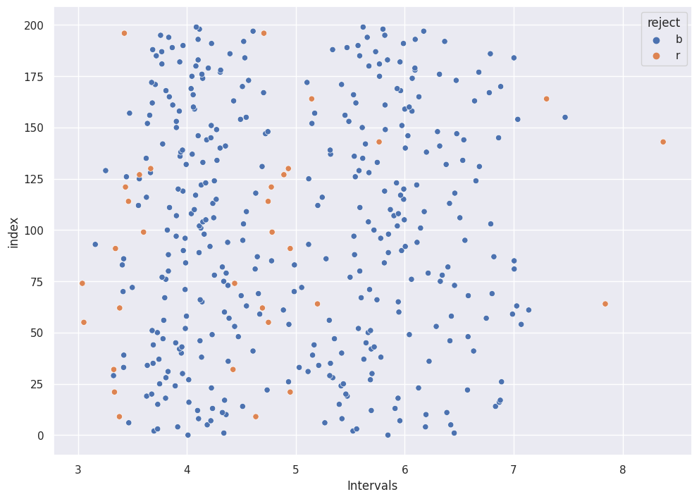
df["reject"].value_counts() / len(df)

b    0.92
r    0.08
Name: reject, dtype: float64