Central Limit Theorem

The Central Limit Theorem (CLT) is a fundamental theorem in probability theory and statistics which states that the sum (or average) of a large number of independent and identically distributed (i.i.d) random variables, each with finite mean and variance, will approximate a normal distribution, regardless of the shape of the original distribution.

Here’s the formal statement:

Given a sequence \(X_1, X_2, X_3, \ldots\) of i.i.d random variables, with each \(X_i\) having the expected value (mean) \(\mu\) and variance \(\sigma^2 < \infty\), the random variables

\[ S_n = \frac{X_1 + X_2 + \ldots + X_n}{n} \]

converges in distribution to a standard normal distribution as \(n\) approaches infinity. This is often expressed as:

\[ \frac{(S_n - \mu)}{\sigma\sqrt{n}} \rightarrow N(0, 1) \]

So what does this mean in layman’s terms? It means that if you were to take a large number of independent random variables from any distribution with a defined mean and variance, then add them up, the distribution of this sum would resemble a normal (bell-shaped) distribution. This outcome still holds true regardless of the original distribution of the variables. It’s one of the key reasons why the normal distribution appears so frequently in statistics and the natural world.

Show code cell content Hide code cell content

from IPython import get_ipython
if get_ipython() is not None:
    get_ipython().run_line_magic('load_ext', 'autoreload')
    get_ipython().run_line_magic('autoreload', '2')
import seaborn as sns; sns.set()
import matplotlib.pyplot as plt
import numpy as np
import pandas as pd
from scipy import stats
sns.set(rc={'figure.figsize':(9,4)})

We often run into odd looking distributions. Take a look at the distribution of fares in the taxi data, shown below. The plot is right skewed with a long tail.

# using taxis dataset from seaborn package
df = sns.load_dataset("taxis")
sns.kdeplot(df['fare'])
print(df['fare'].mean())

13.091072594434944

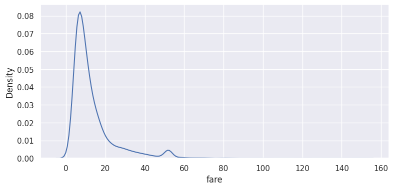
The sample mean of this sample is 13.09.

To construct a sampling distribution, we repeatedly draw samples of size 50; then compute a mean and store it.

def sample_mean(df, n=50):
    sample = np.random.choice(df['fare'], n)
    return np.mean(sample)

means = [sample_mean(df) for i in range(1000)]

Plot this set of sample means:

sns.kdeplot(means)

<Axes: ylabel='Density'>

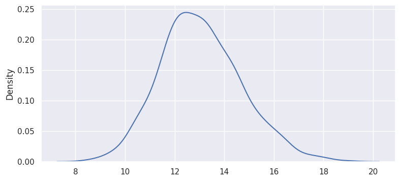
In this example, n=50. In each sample, the sample size was 50 and this step was repeated 1000 times. Central Limit Theorem says that the distribution of sample means converges to a normal distribution as n -> \(\infty\). As a general rule of thumb, sample size should be greater than 30 in order to say the sample mean follows an “approximately normal distribution”.

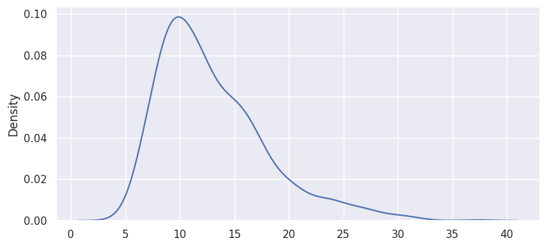
As an example, repeat the same exercise, except with n=5:

means2 = [sample_mean(df, n=5) for i in range(1000)]
sns.kdeplot(means2)

<Axes: ylabel='Density'>

Why is this important? The properties of a normal distribution can be used to conduct hypothesis tests using sample means.

• Suppose you draw a sample of size 50 from some non-normal population and you want to test a hypothesis that the population mean is greater than 10. Central limit theorem and the properties of a normal distribution makes this test possible.

• Similarly, to make inferences using the results of a linear regression, we rely on the normality of the error term and in turn, normality of the parameters. With moderate to large sample sizes, the central limit theorem justifies this assumption.