Discrete Distributions

1. Uniform

2. Hypergeometric

3. Binomial

4. Poisson

5. Geometric

6. Negative Binomial

I try to use examples that can come up in our work. Some of these examples are less cleaner than the standard “balls in an urn or jelly beans” examples that textbooks use.

As an example, fair coin flips are clearly i.i.d. bernoulli trials. Whether a tweet contains hate speech or
not (also binary) is likely not i.i.d.. This is important to keep in mind. In some cases, the i.i.d. assumption may be too strong an assumption and may warrant statistical adjustments.

Show code cell content Hide code cell content

from IPython import get_ipython
if get_ipython() is not None:
    get_ipython().run_line_magic('load_ext', 'autoreload')
    get_ipython().run_line_magic('autoreload', '2')

import seaborn as sns; sns.set()
import matplotlib.pyplot as plt
import numpy as np
import pandas as pd
from scipy import stats
sns.set(rc={'figure.figsize':(9,4)})

Uniform (discrete)

PMF: A random variable X has discrete uniform distribution if

\[P(X=x|N) = \frac{1}{N},\ \ x=1,2,...,N\]

where N is a specified integer.

mean: \(\frac{N+1}{2}\)

var: \(\frac{(N+1)(N-1)}{12}\)

Using stats.randint.rvs to sample from the discrete uniform distribution with N=10:

# https://docs.scipy.org/doc/scipy/reference/generated/scipy.stats.randint.html
# note that scipy.uniform is the continuous uniform distribution
sample = stats.randint.rvs(1,11, size=10000)
print(np.mean(sample))
print(np.var(sample))

5.4749
8.34256999

Hypergeometric

Suppose there are 100 projects at a company and 30 violate a regulation and 70 do not. You collect a sample of 10 projects. What’s the probability that the sample contains 5 violations?

PMF: Let N denote the total population size (30+70=100) and M denote the number of “flagged items” (30 violations). If we let X denote the number of violations in the sample of size K, then X follows a hypergeometric distribution, given by:

\[\begin{split}P(X=x|N,M,K) = \frac{\left(\begin{array}{c} M \\ x\end{array}\right)\left(\begin{array}{c} N-M \\ K-x\end{array}\right)}{\left(\begin{array}{c} N \\ K\end{array}\right)}\end{split}\]

Note:
\(\left(\begin{array}{c} M \\ x\end{array}\right)\) is the combinations to select violations
\(\left(\begin{array}{c} N-M \\ K-x\end{array}\right)\) is the combinations to select non-violations

So in our example:

• N=100

• M=30

• K=10

And so what is P(X=5)?

# https://docs.scipy.org/doc/scipy/reference/reference/generated/scipy.stats.hypergeom.html
[N, K, M] = [100, 30, 10]
rv = stats.hypergeom(N, K, M)
print(rv.pmf(5))

0.09963727785596206

plot the PMF:

[N, K, M] = [100, 30, 10]
rv = stats.hypergeom(N, K, M)
x = np.arange(0, M+1)
pmf = rv.pmf(x)
sns.barplot(x, pmf, color='b')

/home/chansoo/projects/statsbook/.venv/lib/python3.8/site-packages/seaborn/_decorators.py:36: FutureWarning: Pass the following variables as keyword args: x, y. From version 0.12, the only valid positional argument will be `data`, and passing other arguments without an explicit keyword will result in an error or misinterpretation.
  warnings.warn(

<Axes: >

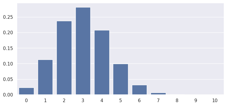
mean: \(\frac{KM}{N}\)
var: \(\frac{KM}{N}\left( \frac{(N-M)(N-K)}{N(N-1)} \right)\)

mean, var, skew, kurt = stats.hypergeom.stats(N, K, M, moments='mvsk')
print(mean)
print(var)

3.0
1.9090909090909092

Binomial

Suppose 25% of a tech company’s content contains misinformation. Since there are millions of posts, the company samples 100 to review. What is the probability that the sample contains 45 misinformation posts?

Quick asides:

• Is 100 too large or too small? To be discussed later in “sampling” section

• But no one knows the true probability. We’ll discuss “hypothesis tests” later which
  can be used to test hypotheses about true probability. Assume 25% rn for demonstration.

• Bayesian methods can also be used where we say company believes probability is 25%. Then update this prior using the data.

First, let’s define a Bernoulli trial. In this example, the trial is whether the post contains misinformation or not. It is a binary variable with probability p (25%) of misinformation:

A random variable X has a \(Bernoulli(p)\) distribution if:

\[\begin{split}X = \left\{ \begin{array}{cc} 1 & \text{with probability}\ p \\ 0 & \text{with probability}\ 1-p \end{array} \right.\end{split}\]

Next, suppose we repeat n Bernoulli trials and define

\[Y = \text{total number of successes (misinformation posts) in}\ n\ \text{trials}\]

Then Y is called a \(binomial(n,p)\) random variable, with this PMF:

\[\begin{split} P(Y = y | n,p) = \left(\begin{array}{c} n \\ y\end{array}\right) p^y(1-p)^{n-y}\end{split}\]

So with p = .25 and n = 100, what is the probability of 45 misinformation posts?

# https://docs.scipy.org/doc/scipy/reference/generated/scipy.stats.binom.html
n, p = 100, 0.25
rv = stats.binom(n,p)
print(rv.pmf(45))

6.6708466821854234e-06

plot the PMF:

x = np.arange(0, 50, step=2)
pmf = rv.pmf(x)
sns.barplot(x, pmf, color='b')

/home/chansoo/projects/statsbook/.venv/lib/python3.8/site-packages/seaborn/_decorators.py:36: FutureWarning: Pass the following variables as keyword args: x, y. From version 0.12, the only valid positional argument will be `data`, and passing other arguments without an explicit keyword will result in an error or misinterpretation.
  warnings.warn(

<Axes: >

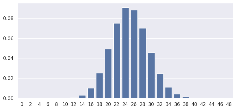
mean: \(np\)
var: \(np(1-p)\)

mean, var, skew, kurt = stats.binom.stats(n, p, moments='mvsk')
print(mean)
print(var)

25.0
18.75

Hypergeometric vs. Binomial

The key difference between these two distributions is the size of the population. In the earlier example for hypergeometric distribution, we considered “violations vs non-violations”. From a population of size 100, we selected a sample of 10 to check for violations. With such a small population and sampling without replacement, note that P(violation) changes with each draw. With 30 violations and 70 non-violations, the p(violation) is 30/100 initially. But if the first sample is a violation, then the p(violation) in the subsequent draw is 29/99.

If the population is large, this change in population can be ignored. Or consider a fair coin flip, which has a hypothetical and infinite population. In these cases, we can use the Binomial distribution. Using the example above, if the population were infinite instead of 100, we would use the Binomial distribution to obtain the probability of X successes given N samples.

Poisson

A Poisson distribution is often used for “waiting-for-occurrence” or “# of hits in an interval”: consider a street intersection that gets one taxi pick-up every 3 hours. What is the probability that there will be no pick-ups in the next 6 hours?

Poisson Relation to Binomial:
Let \(\lambda\) = \(np\). So \(p = \lambda/p\).
Substitute p into the binomial pmf.
Evaluate the limit as n -> \(\infty\) to get the Poisson pmf

PMF: Let \(\lambda\) be the expected hits in an interval, “the intensity parameter”. Then, the probability of X hits in an interval is:

\[P(X=x|\lambda) = \frac{e^{-\lambda}\lambda^x}{x!}\]

Note that one key assumption is that p(hit) is proportional with wait time: The longer we wait, the more likely that there will be a pick-up.

So what is the probability of 0 pickups in 6 hours? We expect 1 pick-up every 3 hours, so we expect 2 pick-ups in 6 hours. Set \(\lambda\) = 2.

# https://docs.scipy.org/doc/scipy/reference/generated/scipy.stats.poisson.html
l = 2
rv = stats.poisson(l)
print(rv.pmf(0))

0.1353352832366127

plot the PMF:

x = np.arange(0, 10)
pmf = rv.pmf(x)
sns.barplot(x, pmf, color='b')

/home/chansoo/projects/statsbook/.venv/lib/python3.8/site-packages/seaborn/_decorators.py:36: FutureWarning: Pass the following variables as keyword args: x, y. From version 0.12, the only valid positional argument will be `data`, and passing other arguments without an explicit keyword will result in an error or misinterpretation.
  warnings.warn(

<Axes: >

mean: \(\lambda\)
var: \(\lambda\)

mean, var, skew, kurt = stats.poisson.stats(l, moments='mvsk')
print(mean)
print(var)

2.0
2.0

Negative Binomial

Suppose that the probability of a success in a task is p = 0.1. While evaluating a sequence of tasks, what’s the probability that the third success is evaluated on the 10th task?

PMF: Let \(X\) denote the task at which the \(r\)th success occurs, where \(r\) is a fixed integer.

Then:

\[\begin{split}p(X=x|r,p) = \left(\begin{array}{c} x-1 \\ r-1\end{array}\right)p^r(1-p)^{x-r}\end{split}\]

Note the relation to the binomial distribution pmf. There are (r) success and x-r failures. We subtract 1 inside the combination since the last trial must be a success.

So with p = 0.1, r = 3, and x = 10:

Note that scipy uses a slightly different, but equivalent PMF: And k denotes the number of failures and n still denotes number of successes. \(p(X=k|n,p) = \left(\begin{array}{c} n+k-1 \\ n-1\end{array}\right)p^n(1-p)^{k}\)

So we want p = 0.1, n = 3, and k = 7:

# https://docs.scipy.org/doc/scipy/reference/generated/scipy.stats.nbinom.html
[n,p] = 3, 0.1
rv = stats.nbinom(n,p)
print(rv.pmf(7))

0.01721868840000001

plot the PMF:

x = np.arange(0, 70, step=2)
pmf = rv.pmf(x)
sns.barplot(x, pmf, color='b')

/home/chansoo/projects/statsbook/.venv/lib/python3.8/site-packages/seaborn/_decorators.py:36: FutureWarning: Pass the following variables as keyword args: x, y. From version 0.12, the only valid positional argument will be `data`, and passing other arguments without an explicit keyword will result in an error or misinterpretation.
  warnings.warn(

<Axes: >

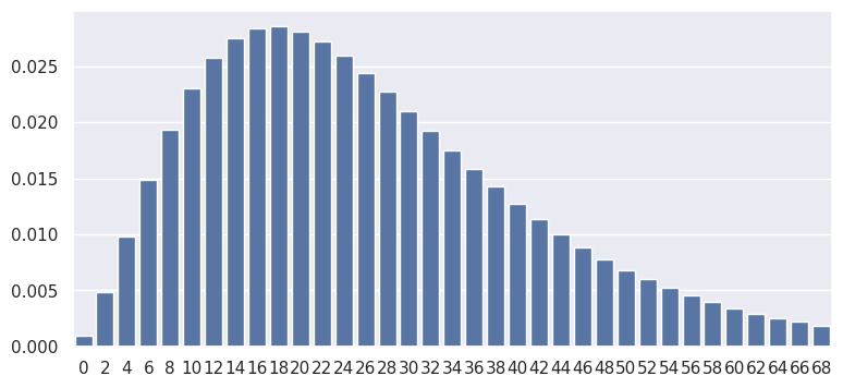
mean: \(r\frac{1-p}{p}\)
var: \(r\frac{1-p}{p^2}\)

mean, var, skew, kurt = stats.nbinom.stats(n, p, moments='mvsk')
print(mean)
print(var)

27.0
269.99999999999994

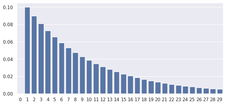
Geometric

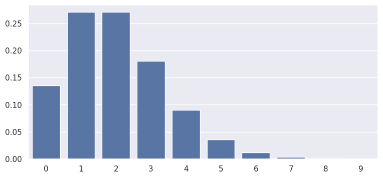
Suppose that the probability of a successes in a task is p = 0.1. What’s the probability that the first two evaluated tasks are fails, then the first successes occurs on the third evaluated task?

PMF: Let Y denote the number of tasks up to and including the first successes.
Then the random variable Y follows a geometric probability distribution if and only if:

\[p(y) = (1-p)^{y-1}p\]

Note the relation to the binomial distribution pmf. There are (y-1) failures and 1 successes. We don’t need to count combinations since the successes must occur on the last trial.

So with p = 0.1 and y = 3:

# https://docs.scipy.org/doc/scipy/reference/generated/scipy.stats.geom.html
p = 0.1
rv = stats.geom(p)
print(rv.pmf(3))

0.08100000000000002

what if we want to know probability that successes occurs on at least the third test?

prob_test_on_first_two = sum([rv.pmf(x) for x in range(3)])
print(1 - prob_test_on_first_two)

0.81

plot the PMF:

x = np.arange(0, 30)
pmf = rv.pmf(x)
sns.barplot(x, pmf, color='b')

/home/chansoo/projects/statsbook/.venv/lib/python3.8/site-packages/seaborn/_decorators.py:36: FutureWarning: Pass the following variables as keyword args: x, y. From version 0.12, the only valid positional argument will be `data`, and passing other arguments without an explicit keyword will result in an error or misinterpretation.
  warnings.warn(

<Axes: >

mean: \(\frac{1}{p}\)
var: \(\frac{1-p}{p^2}\)

mean, var, skew, kurt = stats.geom.stats(p, moments='mvsk')
print(mean)
print(var)

10.0
90.0