P-values#
Show code cell content
from IPython import get_ipython
import numpy as np
np.random.seed(0)
import pandas as pd
from statsmodels.stats.weightstats import ztest
import seaborn as sns
sns.set(rc={'figure.figsize':(11.7,8.27)})
import matplotlib.pyplot as plt
import scipy
import matplotlib.animation as animation
1 test statistic and pvalue#
# one-sided hypothesis test
# NULL Hypothesis: mean = 0
# ALT Hypothesis: mean < 0

# hypothetical population distribution
pop = np.random.normal(-1,2.5,1000)

# what we observe (our sample):
sample_size = 40
sample = np.random.choice(pop, sample_size)
sample_mean = np.mean(sample)
sample_var = np.var(sample)
test_statistic = (sample_mean - 0) / np.sqrt(sample_var/(sample_size-1))
pvalue = 1-scipy.stats.norm.cdf(abs(test_statistic), 0, 1)
print(test_statistic, pvalue)
-2.894948524449533 0.0018961035676138271
# equivalently, using statsmodels' ztest:
test_statistic, pvalue = ztest(sample, value=0, alternative='smaller')
print(test_statistic, pvalue)
-2.894948524449533 0.0018961035676138293
2 distributions of test statistics and pvalues#
def sim(pop, sample_size = 40):
    sample = np.random.choice(pop, sample_size)
    sample_mean = np.mean(sample)
    sample_var = np.var(sample)
    test_statistic = (sample_mean - 0) / np.sqrt(sample_var/(sample_size-1))
    pvalue = scipy.stats.norm.cdf(test_statistic, 0, 1)
    return pvalue, test_statistic

std_normal = np.random.normal(0,1,100_000)

results = pd.DataFrame([
    sim(pop, 40)
    for i in range(1000)
], columns=["pvalue", "test_statistic"])
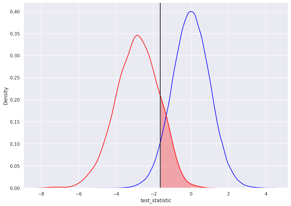
First couple plots address questions we had about the distribution of pvalues under repeated sampling.
The blue distribution is just a standard normal distribution (mean=0, variance=1).
The orange distribution is a distribution of 1000 simulated test statistics from repeated experiments.
The black line represents the researcher’s decision to select alpha = 0.05.
We reject the null for test statistics that are shaded in red.
ax = sns.kdeplot(std_normal, color="blue")
ax = sns.kdeplot(results["test_statistic"], color="red")
plt.axvline(-1.645, 0, 1, color="black")
l1 = ax.lines[0]
l2 = ax.lines[1]
x1 = l1.get_xydata()[:,0]
y1 = l1.get_xydata()[:,1]
x2 = l2.get_xydata()[:,0]
y2 = l2.get_xydata()[:,1]
ax.fill_between(x2[x2<-1.645],y2[x2<-1.645], color="red", alpha=0.3)
<matplotlib.collections.PolyCollection at 0x7fa361d65b20>
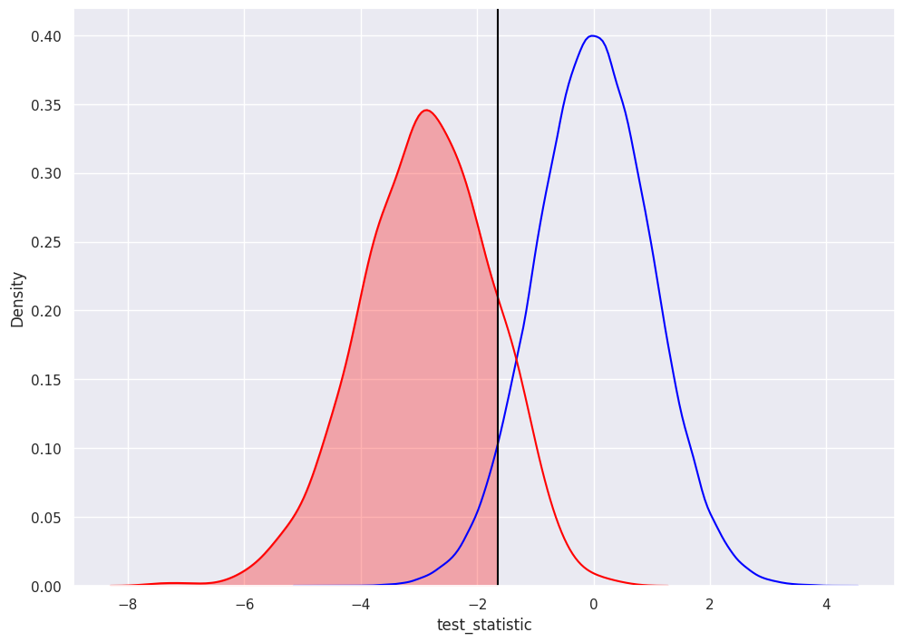
for this data, using an alpha=0.05, about 86% of test statistics are statistically significantly different from zero (less than -1.645)
np.mean([results["test_statistic"]<-1.645])
0.855
each of these test statistics has its own pvalue
sns.histplot(results["pvalue"], bins=100)
plt.axvline(0.05, 0, 1000, color="red")
<matplotlib.lines.Line2D at 0x7fa361d1d310>
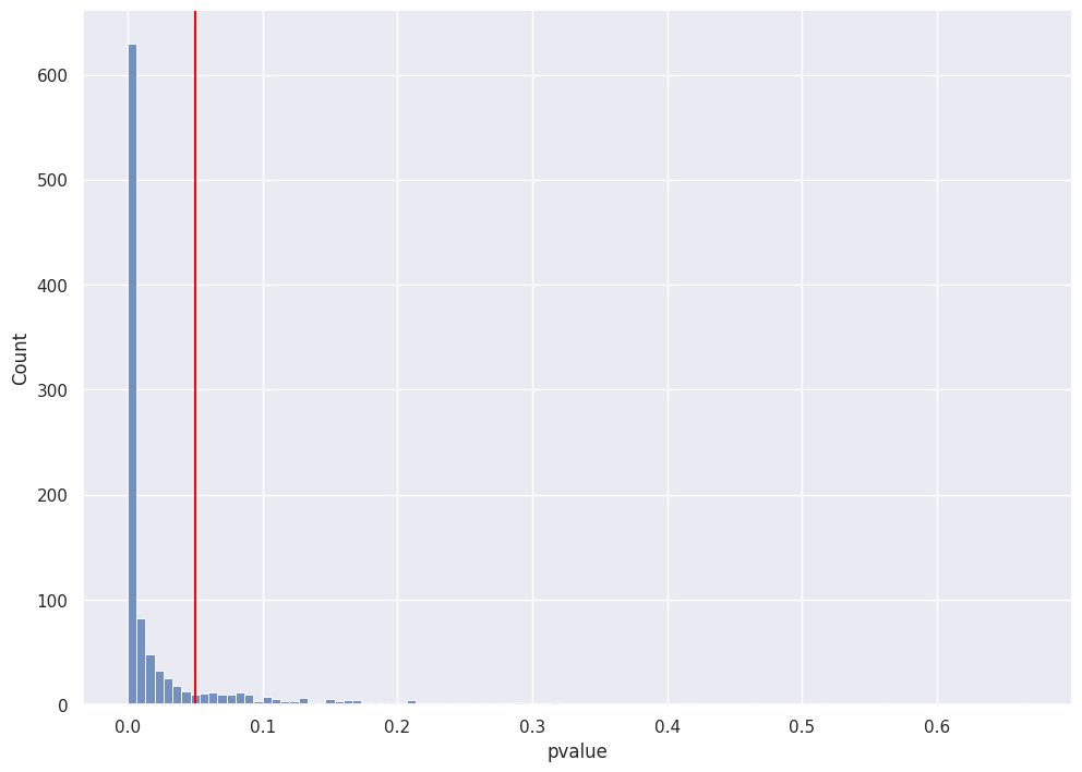
again, ~86% of simulated pvalues are below 0.05 (equivalent to 86% of test statistics > 1.645)
np.mean([results["pvalue"]<0.05])
0.855
we’ll see below, but this value 86% is closely related to type 2 error and is called power of a test
type 1 error and alpha#
type 1 error occurs when we reject the null when it is true.
alpha is the probability of a type 1 error.
here, the researcher selected an alpha of 0.05, so the rejection decision is to reject all test statistics less than -1.645 (black vertical line) equivalently, to reject all pvalues less than 0.05.
the shaded area in red represents 5% of the area under the blue distribution
1 - alpha is our confidence level
ax = sns.kdeplot(std_normal, color="blue")
ax = sns.kdeplot(results["test_statistic"], color="red")
plt.axvline(-1.645, 0, 1, color="black")
l1 = ax.lines[0]
l2 = ax.lines[1]
x1 = l1.get_xydata()[:,0]
y1 = l1.get_xydata()[:,1]
x2 = l2.get_xydata()[:,0]
y2 = l2.get_xydata()[:,1]
ax.fill_between(x1[x1<-1.645],y1[x1<-1.645], color="red", alpha=0.3)
<matplotlib.collections.PolyCollection at 0x7fa361bad9a0>
as we expect with a standard normal distribution and by design (since researcher selected alpha), the we can confirm shaded area represents 5% of blue distribution:
np.mean([std_normal<-1.645])
0.04964
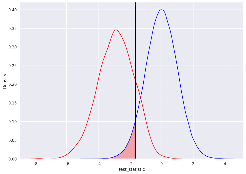
type 2 error and beta#
type 2 error is failing to reject the null when it is actually false
beta is the probability of a type 2 error
again, researcher selected the alpha of 0.05… so the rejection decision is to NOT reject test statistics greater than -1.645
the shaded area in red represents a percentage of the red distribution (we computed the area under the red distribution BELOW -1.645 earlier, so this is just 1 minus that value): 1 - .86 = 14%
1 - beta is the “power of the test”, it’s the probability that the test correctly rejects the null (the percentage of pvalues less than -1.645)
ax = sns.kdeplot(std_normal, color="blue")
ax = sns.kdeplot(results["test_statistic"], color="red")
plt.axvline(-1.645, 0, 1, color="black")
l1 = ax.lines[0]
l2 = ax.lines[1]
x1 = l1.get_xydata()[:,0]
y1 = l1.get_xydata()[:,1]
x2 = l2.get_xydata()[:,0]
y2 = l2.get_xydata()[:,1]
ax.fill_between(x2[x2>-1.645],y2[x2>-1.645], color="red", alpha=0.3)
<matplotlib.collections.PolyCollection at 0x7fa361ad2100>
to confirm:
np.mean(results["test_statistic"]>-1.645)
0.145
animations#
when null is true#
population mean is equal to our hypothesis (mean = 0)
np.random.seed(0)
pop = np.random.normal(0,1,1000)
results = pd.DataFrame([
    sim(pop, 40)
    for i in range(1000)
], columns=["pvalue", "test_statistic"])
if get_ipython() is not None:
    get_ipython().run_line_magic('matplotlib', 'ipympl')

fig, (ax1,ax2,ax3) = plt.subplots(3,1)
fig.set_size_inches(8, 11.5, True)

def init():
    sns.ecdfplot(std_normal, ax=ax2, color="blue")

def animate(frame_number):
    ax1.clear()
    ax3.clear()

    sns.kdeplot(std_normal, color="blue", ax=ax1)
    sns.kdeplot(results["test_statistic"], color="red", ax=ax1)
    l2 = ax1.lines[1]
    x2 = l2.get_xydata()[:,0]
    y2 = l2.get_xydata()[:,1]
    teststat = results["test_statistic"][frame_number]
    ax1.axvline(teststat, 0, 1, color="green")
    ax1.fill_between(x1[x1<teststat],y1[x1<teststat], color="red", alpha=0.3)
    ax1.text(0.5,1.1,
        f"Simulation {frame_number} out of 100",
        bbox={'facecolor':'w', 'alpha':0.5, 'pad':5},
        transform=ax1.transAxes,
        ha="center",
        weight='bold',
        size=12
    )

    pvalue = results["pvalue"][frame_number]
    ax2.axhline(pvalue,-10,10, color="green")
    ax2.set_xlabel('test_statistic')
    ax2.set_ylabel('pvalue')

    sns.histplot(results["pvalue"][:frame_number], color="green", ax=ax3)

ani = animation.FuncAnimation(
    fig,
    animate,
    frames=100,
    init_func=init,
    repeat=False,
    blit=True,
    interval=100
)

# writergif = animation.PillowWriter(fps=2)
# ani.save('null_true.gif', writer=writergif)
Show code cell output
when null is NOT true#
population mean is NOT equal to our hypothesis (mean = 0)
pop = np.random.normal(-1,2,1000)
results = pd.DataFrame([
    sim(pop, 40)
    for i in range(1000)
], columns=["pvalue", "test_statistic"])
if get_ipython() is not None:
    get_ipython().run_line_magic('matplotlib', 'ipympl')

fig, (ax1,ax2,ax3) = plt.subplots(3,1)
fig.set_size_inches(8, 11.5, True)

def init():
    sns.ecdfplot(std_normal, ax=ax2, color="blue")

def animate(frame_number):
    ax1.clear()
    ax3.clear()

    sns.kdeplot(std_normal, color="blue", ax=ax1)
    sns.kdeplot(results["test_statistic"], color="red", ax=ax1)
    l2 = ax1.lines[1]
    x2 = l2.get_xydata()[:,0]
    y2 = l2.get_xydata()[:,1]
    teststat = results["test_statistic"][frame_number]
    ax1.axvline(teststat, 0, 1, color="green")
    ax1.fill_between(x1[x1<teststat],y1[x1<teststat], color="red", alpha=0.3)
    ax1.text(0.5,1.1,
        f"Simulation {frame_number} out of 100",
        bbox={'facecolor':'w', 'alpha':0.5, 'pad':5},
        transform=ax1.transAxes,
        ha="center",
        weight='bold',
        size=12
    )

    pvalue = results["pvalue"][frame_number]
    ax2.axhline(pvalue,-10,10, color="green")
    ax2.set_xlabel('test_statistic')
    ax2.set_ylabel('pvalue')

    sns.histplot(results["pvalue"][:frame_number], color="green", ax=ax3)

ani = animation.FuncAnimation(
    fig,
    animate,
    frames=100,
    init_func=init,
    repeat=False,
    blit=True,
    interval=100
)

# writergif = animation.PillowWriter(fps=2)
# ani.save('null_not_true.gif', writer=writergif)
Show code cell output
/home/chansoo/projects/statsbook/.venv/lib/python3.8/site-packages/matplotlib/animation.py:884: UserWarning: Animation was deleted without rendering anything. This is most likely not intended. To prevent deletion, assign the Animation to a variable, e.g. `anim`, that exists until you output the Animation using `plt.show()` or `anim.save()`.
  warnings.warn(