Multivariate Distributions

Key concepts for this section:

1. Correlation / covariance

2. Contingency Table

3. Plotting joint/conditional/marginal distributions

4. Simpson’s paradox, confounder?

Show code cell content Hide code cell content

from IPython import get_ipython
if get_ipython() is not None:
    get_ipython().run_line_magic('load_ext', 'autoreload')
    get_ipython().run_line_magic('autoreload', '2')

import seaborn as sns; sns.set()
import matplotlib.pyplot as plt
import numpy as np
import pandas as pd
from scipy import stats
sns.set(rc={'figure.figsize':(9,4)})

# Fake Data:
n=100
df = pd.DataFrame({
    "a":np.random.normal(10, 1, n),
})
df["c"] = df["a"] + np.random.normal(1, 0.5, n)

Correlation / Covariance

Covariance indicates the level to which two variables vary together.

\[Cov(X,Y) = \frac{1}{n}\sum_{i=1}^n(x_i - E(X))(y_i-E(Y))\]

# Compute covariance manually:
products = [
    (row["a"]-df["a"].mean()) * (row["c"]-df["c"].mean())
    for i,row in df.iterrows()
]
covariance = np.sum(products)/len(df)
print(covariance)

1.2540311514944218

# Using numpy:
# if bias = False, computes "sample covariance" so denominator is N-1
np.cov(df["a"], df["c"], bias=True)

array([[1.25936321, 1.25403115],
       [1.25403115, 1.46689568]])

Pearson correlation coefficient is the covariance divided by product of standard deviations

\[\rho_{X,Y} = \frac{cov(X,Y)}{\sigma_X\sigma_Y}\]

also see: spearman’s rank correlation coefficient

corr = covariance / (np.std(df["a"]) * np.std(df["c"]))
corr

0.9226419733025584

np.corrcoef(df["a"], df["c"])

array([[1.        , 0.92264197],
       [0.92264197, 1.        ]])

Contingency Table

df_cat = pd.DataFrame({
    "colors":np.random.choice(["red","blue","green","yellow","orange"], size=30, replace=True),
    "names":np.random.choice(["jason","jorge","lisa","paul"], size=30, replace=True),
    "states":np.random.choice(["california","arizona","oregon"], size=30, replace=True),
})

pd.crosstab(
    [df_cat["states"],df_cat["names"]], 
    df_cat["colors"], 
    margins=True
)

	colors	blue	green	orange	red	yellow	All
states	names
arizona	jason	1	0	1	0	1	3
	jorge	0	0	0	0	1	1
	lisa	0	0	0	1	0	1
	paul	3	0	0	1	0	4
california	jason	0	0	1	1	1	3
	jorge	1	0	0	1	1	3
	lisa	0	2	0	1	1	4
	paul	0	0	1	1	1	3
oregon	jason	0	1	1	1	1	4
	lisa	1	0	1	2	0	4
All		6	3	5	9	7	30

pd.crosstab(
    [df_cat["states"],df_cat["names"]], df_cat["colors"], 
    margins=True, 
    normalize=True
)

	colors	blue	green	orange	red	yellow	All
states	names
arizona	jason	0.033333	0.000000	0.033333	0.000000	0.033333	0.100000
	jorge	0.000000	0.000000	0.000000	0.000000	0.033333	0.033333
	lisa	0.000000	0.000000	0.000000	0.033333	0.000000	0.033333
	paul	0.100000	0.000000	0.000000	0.033333	0.000000	0.133333
california	jason	0.000000	0.000000	0.033333	0.033333	0.033333	0.100000
	jorge	0.033333	0.000000	0.000000	0.033333	0.033333	0.100000
	lisa	0.000000	0.066667	0.000000	0.033333	0.033333	0.133333
	paul	0.000000	0.000000	0.033333	0.033333	0.033333	0.100000
oregon	jason	0.000000	0.033333	0.033333	0.033333	0.033333	0.133333
	lisa	0.033333	0.000000	0.033333	0.066667	0.000000	0.133333
All		0.200000	0.100000	0.166667	0.300000	0.233333	1.000000

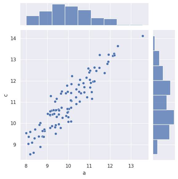
Joint / Conditional / Marginal Distributions

joint distribution

\[f(a,c)\]

sns.jointplot(df["a"],df["c"])

/home/chansoo/projects/statsbook/.venv/lib/python3.8/site-packages/seaborn/_decorators.py:36: FutureWarning: Pass the following variables as keyword args: x, y. From version 0.12, the only valid positional argument will be `data`, and passing other arguments without an explicit keyword will result in an error or misinterpretation.
  warnings.warn(

<seaborn.axisgrid.JointGrid at 0x7f3518532640>

conditional distribution

\[f(a|c>0)\]

sns.kdeplot(df.loc[df["c"]>0,"a"])

<Axes: xlabel='a', ylabel='Density'>

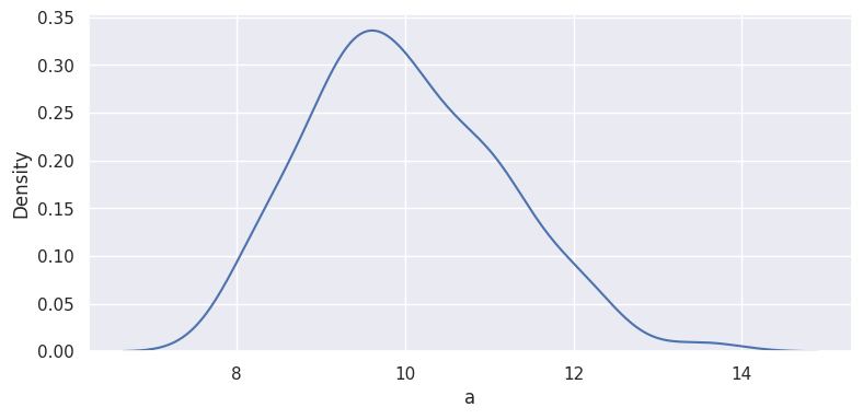
marginal distribution

\[f(a)\]

sns.kdeplot(df["a"])

<Axes: xlabel='a', ylabel='Density'>

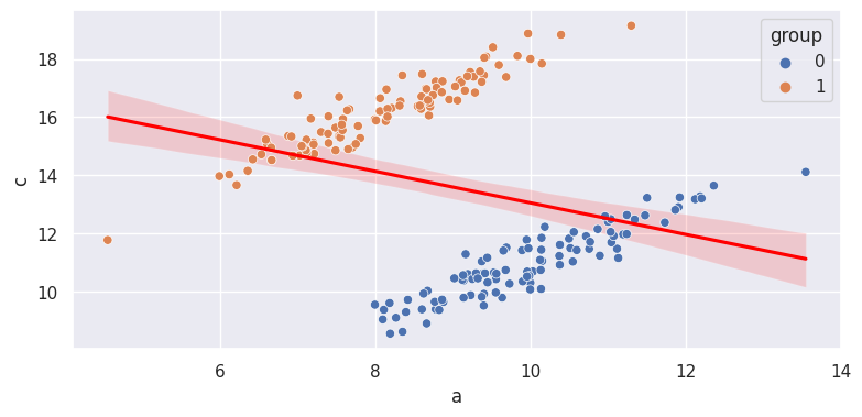
Simpson’s Paradox

df2 = pd.DataFrame({
    "a":np.random.normal(8, 1, n),
})
df2["c"] = df2["a"] + np.random.normal(8, 0.5, n)
df["group"] = 0
df2["group"] = 1
df_simpson = pd.concat([df[["a","c","group"]],df2])

sns.regplot(df_simpson["a"], df_simpson["c"], scatter=False, color="red")
sns.scatterplot(df_simpson["a"], df_simpson["c"], hue=df_simpson["group"])

/home/chansoo/projects/statsbook/.venv/lib/python3.8/site-packages/seaborn/_decorators.py:36: FutureWarning: Pass the following variables as keyword args: x, y. From version 0.12, the only valid positional argument will be `data`, and passing other arguments without an explicit keyword will result in an error or misinterpretation.
  warnings.warn(

<Axes: xlabel='a', ylabel='c'>