Interactions#
import numpy as np
import pandas as pd
import statsmodels.api as sm
import seaborn as sns
import patsy
from matplotlib import pyplot as plt
from scipy.special import expit as invlogit
OLS#
n = 500
np.random.seed(0)
df = pd.DataFrame({
    "income":np.random.normal(5,1,n),
    # "educ":np.random.choice([1,2,3,4,5], n),
    "e":np.random.normal(0,1,n)
})

df["educ"] = 1 + np.random.binomial(4,df["income"] / df["income"].max())

df["favorability"] = 2 + 1.4*df["income"] + 5*df["educ"] + -0.9*df["income"]*df["educ"] + df["e"]
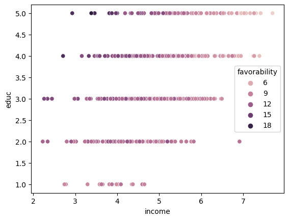
sns.scatterplot(df["income"],df["educ"], hue=df["favorability"])
/home/chansoo/projects/statsbook/.venv/lib/python3.8/site-packages/seaborn/_decorators.py:36: FutureWarning: Pass the following variables as keyword args: x, y. From version 0.12, the only valid positional argument will be `data`, and passing other arguments without an explicit keyword will result in an error or misinterpretation.
  warnings.warn(
<Axes: xlabel='income', ylabel='educ'>
f = 'favorability ~ income + C(educ) + income*C(educ)'
y, X = patsy.dmatrices(f, df, return_type='dataframe')
mod = sm.OLS(y, X)
res = mod.fit()
print(res.summary())
                            OLS Regression Results
==============================================================================
Dep. Variable:           favorability   R-squared:                       0.804
Model:                            OLS   Adj. R-squared:                  0.801
Method:                 Least Squares   F-statistic:                     224.0
Date:                Thu, 01 Jun 2023   Prob (F-statistic):          2.19e-167
Time:                        12:45:57   Log-Likelihood:                -694.78
No. Observations:                 500   AIC:                             1410.
Df Residuals:                     490   BIC:                             1452.
Df Model:                           9
Covariance Type:            nonrobust
=======================================================================================
                          coef    std err          t      P>|t|      [0.025      0.975]
---------------------------------------------------------------------------------------
Intercept               8.2033      1.758      4.666      0.000       4.749      11.658
C(educ)[T.2]            3.6147      1.851      1.953      0.051      -0.022       7.251
C(educ)[T.3]            8.7862      1.823      4.821      0.000       5.205      12.367
C(educ)[T.4]           13.9905      1.813      7.718      0.000      10.429      17.552
C(educ)[T.5]           18.6545      1.847     10.102      0.000      15.026      22.283
income                  0.1805      0.455      0.397      0.691      -0.713       1.074
income:C(educ)[T.2]    -0.5144      0.473     -1.087      0.278      -1.444       0.416
income:C(educ)[T.3]    -1.4917      0.465     -3.207      0.001      -2.406      -0.578
income:C(educ)[T.4]    -2.4434      0.462     -5.285      0.000      -3.352      -1.535
income:C(educ)[T.5]    -3.2722      0.465     -7.034      0.000      -4.186      -2.358
==============================================================================
Omnibus:                        0.246   Durbin-Watson:                   2.091
Prob(Omnibus):                  0.884   Jarque-Bera (JB):                0.166
Skew:                           0.041   Prob(JB):                        0.920
Kurtosis:                       3.035   Cond. No.                         543.
==============================================================================

Notes:
[1] Standard Errors assume that the covariance matrix of the errors is correctly specified.
The above example is fake data containing favorability ratings for some politician. Each row is a constituent and covariates measure their level of education (categorical variable from 1 to 5) and their income (in 10k).
Interpretations:
The intercept represents the favorability rating for an individual with education level 1 and 0 income.
The coefficient of C(educ)[T.d] represents the average difference in favorability rating between an individual with education level 1 and education level 2 for an individual with income = 0.
The coefficient of income represents the average change in favorability given a one unit increase (10k increase) in income for an individual with edcuation level = 0.
If there were no interaction term, this coefficient would represent a change in favorability given a one unit increase in income for any individual, regardless of income. But due to interactions, this coefficient can only be interpreted for an individual with education level = 0.
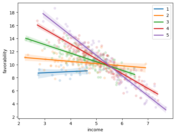
The coefficient of “income:C(educ)[T.2]” represents the average difference in the slope of the relationship between income and favorability, when between an individual with education level 1 vs education level 2. This coefficient can also be interpreted as the average change in differences between an education level 1 vs level 2, for a one unit increase in income. Here, a coefficient of -0.5144 suggests that the slope of income on favorability is 0.1805 for education level 1 individuals and 0.1805-0.5144=-0.3339 for education level 2. Another interpretation would be that for every one unit increase in income, the gap in favorability between education level 1 and education level 2 (3.6147), decreases by -0.5144.
def plot_scatter(df,educ):
    g = sns.scatterplot("income","favorability",data=df.query(f"educ=={educ}"), alpha=0.2)
    g = sns.regplot("income","favorability",data=df.query(f"educ=={educ}"), label=educ, scatter=False)
    return g

for educ in range(1,6):
    g1 = plot_scatter(df,educ)
g1.legend()
/home/chansoo/projects/statsbook/.venv/lib/python3.8/site-packages/seaborn/_decorators.py:36: FutureWarning: Pass the following variables as keyword args: x, y. From version 0.12, the only valid positional argument will be `data`, and passing other arguments without an explicit keyword will result in an error or misinterpretation.
  warnings.warn(
<matplotlib.legend.Legend at 0x7fd2141e30d0>
Centering#
Whether fitting an OLS, GLM, or MLM, centering can help with easier interpretation when interactions are present.
df["income_ctr"] = df["income"] - np.mean(df["income"])
f = 'favorability ~ income_ctr + C(educ) + income_ctr*C(educ)'
y, X = patsy.dmatrices(f, df, return_type='dataframe')
mod = sm.OLS(y, X)
res = mod.fit()
print(res.summary())
                            OLS Regression Results
==============================================================================
Dep. Variable:           favorability   R-squared:                       0.804
Model:                            OLS   Adj. R-squared:                  0.801
Method:                 Least Squares   F-statistic:                     224.0
Date:                Thu, 01 Jun 2023   Prob (F-statistic):          2.19e-167
Time:                        12:45:58   Log-Likelihood:                -694.78
No. Observations:                 500   AIC:                             1410.
Df Residuals:                     490   BIC:                             1452.
Df Model:                           9
Covariance Type:            nonrobust
===========================================================================================
                              coef    std err          t      P>|t|      [0.025      0.975]
-------------------------------------------------------------------------------------------
Intercept                   9.1013      0.580     15.697      0.000       7.962      10.241
C(educ)[T.2]                1.0560      0.597      1.768      0.078      -0.118       2.230
C(educ)[T.3]                1.3657      0.586      2.332      0.020       0.215       2.516
C(educ)[T.4]                1.8355      0.585      3.137      0.002       0.686       2.985
C(educ)[T.5]                2.3766      0.592      4.017      0.000       1.214       3.539
income_ctr                  0.1805      0.455      0.397      0.691      -0.713       1.074
income_ctr:C(educ)[T.2]    -0.5144      0.473     -1.087      0.278      -1.444       0.416
income_ctr:C(educ)[T.3]    -1.4917      0.465     -3.207      0.001      -2.406      -0.578
income_ctr:C(educ)[T.4]    -2.4434      0.462     -5.285      0.000      -3.352      -1.535
income_ctr:C(educ)[T.5]    -3.2722      0.465     -7.034      0.000      -4.186      -2.358
==============================================================================
Omnibus:                        0.246   Durbin-Watson:                   2.091
Prob(Omnibus):                  0.884   Jarque-Bera (JB):                0.166
Skew:                           0.041   Prob(JB):                        0.920
Kurtosis:                       3.035   Cond. No.                         42.2
==============================================================================

Notes:
[1] Standard Errors assume that the covariance matrix of the errors is correctly specified.
Note the change in the coefficients for the interaction terms.
Now, the coefficient for C(educ)[T.2], 1.0560, is the change in favorability
between an individual with educ=1 and educ=2, with average income level.
(as opposed to income = 0)
Logistic#
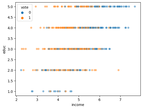
Now, we generate a binary “vote” column.
Then we model the probability of vote using a logit link.
df["vote"] = np.random.binomial(1, invlogit(df["favorability"]-np.mean(df["favorability"])), n)
sns.scatterplot("income","educ",hue="vote", data=df, alpha=0.5)
/home/chansoo/projects/statsbook/.venv/lib/python3.8/site-packages/seaborn/_decorators.py:36: FutureWarning: Pass the following variables as keyword args: x, y. From version 0.12, the only valid positional argument will be `data`, and passing other arguments without an explicit keyword will result in an error or misinterpretation.
  warnings.warn(
<Axes: xlabel='income', ylabel='educ'>
f = 'vote ~ income + C(educ) + income*C(educ)'
y, X = patsy.dmatrices(f, df, return_type='dataframe')
mod = sm.Logit(y, X)
res_log = mod.fit()
print(res_log.summary())
Optimization terminated successfully.
         Current function value: 0.524547
         Iterations 7
                           Logit Regression Results
==============================================================================
Dep. Variable:                   vote   No. Observations:                  500
Model:                          Logit   Df Residuals:                      490
Method:                           MLE   Df Model:                            9
Date:                Thu, 01 Jun 2023   Pseudo R-squ.:                  0.2404
Time:                        12:45:58   Log-Likelihood:                -262.27
converged:                       True   LL-Null:                       -345.28
Covariance Type:            nonrobust   LLR p-value:                 4.187e-31
=======================================================================================
                          coef    std err          z      P>|z|      [0.025      0.975]
---------------------------------------------------------------------------------------
Intercept              -4.4793      5.175     -0.866      0.387     -14.622       5.663
C(educ)[T.2]            4.5777      5.311      0.862      0.389      -5.831      14.986
C(educ)[T.3]           10.2035      5.343      1.910      0.056      -0.269      20.676
C(educ)[T.4]           14.9313      5.427      2.751      0.006       4.294      25.569
C(educ)[T.5]           18.8533      5.956      3.165      0.002       7.179      30.527
income                  0.7932      1.294      0.613      0.540      -1.743       3.329
income:C(educ)[T.2]    -0.7420      1.322     -0.561      0.575      -3.334       1.849
income:C(educ)[T.3]    -1.8763      1.321     -1.421      0.155      -4.465       0.712
income:C(educ)[T.4]    -2.7696      1.331     -2.081      0.037      -5.378      -0.161
income:C(educ)[T.5]    -3.4311      1.399     -2.453      0.014      -6.173      -0.689
=======================================================================================
And the model after centering:
f = 'vote ~ income_ctr + C(educ) + income_ctr*C(educ)'
y, X = patsy.dmatrices(f, df, return_type='dataframe')
mod = sm.Logit(y, X)
res_log = mod.fit()
print(res_log.summary())
Optimization terminated successfully.
         Current function value: 0.524547
         Iterations 7
                           Logit Regression Results
==============================================================================
Dep. Variable:                   vote   No. Observations:                  500
Model:                          Logit   Df Residuals:                      490
Method:                           MLE   Df Model:                            9
Date:                Thu, 01 Jun 2023   Pseudo R-squ.:                  0.2404
Time:                        12:45:58   Log-Likelihood:                -262.27
converged:                       True   LL-Null:                       -345.28
Covariance Type:            nonrobust   LLR p-value:                 4.187e-31
===========================================================================================
                              coef    std err          z      P>|z|      [0.025      0.975]
-------------------------------------------------------------------------------------------
Intercept                  -0.5332      1.458     -0.366      0.715      -3.391       2.324
C(educ)[T.2]                0.8864      1.488      0.596      0.551      -2.030       3.803
C(educ)[T.3]                0.8695      1.469      0.592      0.554      -2.010       3.749
C(educ)[T.4]                1.1536      1.474      0.783      0.434      -1.734       4.042
C(educ)[T.5]                1.7848      1.514      1.179      0.238      -1.182       4.752
income_ctr                  0.7932      1.294      0.613      0.540      -1.743       3.329
income_ctr:C(educ)[T.2]    -0.7420      1.322     -0.561      0.575      -3.334       1.849
income_ctr:C(educ)[T.3]    -1.8763      1.321     -1.421      0.155      -4.465       0.712
income_ctr:C(educ)[T.4]    -2.7696      1.331     -2.081      0.037      -5.378      -0.161
income_ctr:C(educ)[T.5]    -3.4311      1.399     -2.453      0.014      -6.173      -0.689
===========================================================================================
Interpretations:
The intercept coefficient is -0.8973 before centering and 1.36 after centering. Before centering, this means that a voter with educ=1 and income=0 has a \(logit^{-1}(-0.8973) = 0.29\) probability of voting yes. After centering, this means that the voter with educ=1 and average income has a \(logit^{-1}(-0.2587) = 0.44\) probability of voting yes.
In the centered model, the coefficient for C(educ)[T.2] is 0.1327. For an individual with average income, the individual with educ=2 has \(logit^{-1}(-0.2587+0.1327) = 0.46\) probability of voting, a decrease of ~0.02 from 0.44.
In the centered model, the coefficient for C(educ)[T.2] is 0.1327. For an individual with average income, the individual with educ=2 has \(logit^{-1}(-0.2587+0.1327) = 0.46\) probability of voting, a decrease of ~0.02 from 0.44.
invlogit(-0.8973)
0.2896056640703297
invlogit(-0.2587)
0.4356833038013948
invlogit(0.1327)
0.5331264032240327
invlogit(-0.2587+0.1327)
0.46854160844368314
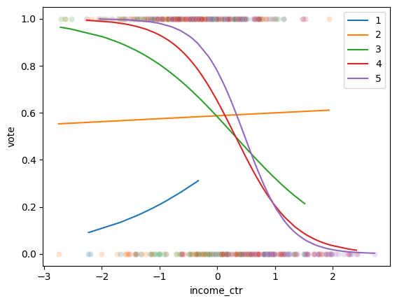
To compare individuals with income 0.5 below the mean, -0.5, and education = 3 vs individuals with income -0.5 and education = 5
Then compare with income = 1.
Verify in plots below.
income = -0.5
print(invlogit(-0.2587 + 0.8255 + 0.1284 * income + -1.0049*income))
print(invlogit(-0.2587 + 0.9480 + 0.1284 * income +  -2.8437*income))
0.7320503095881152
0.885639070225958
income = 1
print(invlogit(-0.2587 + 0.8255 + 0.1284 * income + -1.0049*income))
print(invlogit(-0.2587 + 0.9480 + 0.1284 * income +  -2.8437*income))
0.4231879671534434
0.11650000193030657
df["pred"] = res_log.predict()
def plot_scatter(df,educ):
    g = sns.scatterplot("income_ctr","vote",data=df.query(f"educ=={educ}"), alpha=0.2)
    g = sns.lineplot("income_ctr","pred",data=df.query(f"educ=={educ}"), label=educ)
    return g

for educ in range(1,6):
    g1 = plot_scatter(df,educ)
g1.legend()
/home/chansoo/projects/statsbook/.venv/lib/python3.8/site-packages/seaborn/_decorators.py:36: FutureWarning: Pass the following variables as keyword args: x, y. From version 0.12, the only valid positional argument will be `data`, and passing other arguments without an explicit keyword will result in an error or misinterpretation.
  warnings.warn(
/home/chansoo/projects/statsbook/.venv/lib/python3.8/site-packages/seaborn/_decorators.py:36: FutureWarning: Pass the following variables as keyword args: x, y. From version 0.12, the only valid positional argument will be `data`, and passing other arguments without an explicit keyword will result in an error or misinterpretation.
  warnings.warn(
/home/chansoo/projects/statsbook/.venv/lib/python3.8/site-packages/seaborn/_decorators.py:36: FutureWarning: Pass the following variables as keyword args: x, y. From version 0.12, the only valid positional argument will be `data`, and passing other arguments without an explicit keyword will result in an error or misinterpretation.
  warnings.warn(
/home/chansoo/projects/statsbook/.venv/lib/python3.8/site-packages/seaborn/_decorators.py:36: FutureWarning: Pass the following variables as keyword args: x, y. From version 0.12, the only valid positional argument will be `data`, and passing other arguments without an explicit keyword will result in an error or misinterpretation.
  warnings.warn(
/home/chansoo/projects/statsbook/.venv/lib/python3.8/site-packages/seaborn/_decorators.py:36: FutureWarning: Pass the following variables as keyword args: x, y. From version 0.12, the only valid positional argument will be `data`, and passing other arguments without an explicit keyword will result in an error or misinterpretation.
  warnings.warn(
/home/chansoo/projects/statsbook/.venv/lib/python3.8/site-packages/seaborn/_decorators.py:36: FutureWarning: Pass the following variables as keyword args: x, y. From version 0.12, the only valid positional argument will be `data`, and passing other arguments without an explicit keyword will result in an error or misinterpretation.
  warnings.warn(
<matplotlib.legend.Legend at 0x7fd2141e3310>