WLS#
Use Cases:
Using observed data to represent a larger population: Suppose you are using a sample from a survey that oversampled from some groups. We could use the survey weights in a WLS to minimize SSE with respect to the population instead of the sample. Let \(\pi_g\) be the population share of group g. And let \(h_g\) be the sample share of group G. Then define weight for unit i to be \(w_i\) as \(\frac{pi_{gi}}{h_{gi}}\).
duplicate observations (or aggregated data): if observations with covariates {X_i} appear multiple times, you could include these observations just once and set \(w_i\) to be the number of times they appear.
Unequal variance: if there is a lot of heteroskeasticity, you can set weights to the inverse of the error variance
import numpy as np
import pandas as pd
import statsmodels.api as sm
import seaborn as sns
import patsy
# create two groups for error variance, low and high
n = 300
np.random.seed(0)
df = pd.DataFrame({
"x1":np.random.normal(10,1,n),
"e":np.random.normal(0,1,n)
}).sort_values('x1')
sigma = 0.5
w = np.ones(n)
w = df["x1"] / 2
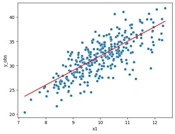
df["y_true"] = 2 + 3*df["x1"]
df["y_obs"] = df["y_true"] + w*sigma*df["e"]
sns.scatterplot(df["x1"], df["y_obs"])
sns.lineplot(df["x1"], df["y_true"], color="red")
/home/chansoo/projects/statsbook/.venv/lib/python3.8/site-packages/seaborn/_decorators.py:36: FutureWarning: Pass the following variables as keyword args: x, y. From version 0.12, the only valid positional argument will be `data`, and passing other arguments without an explicit keyword will result in an error or misinterpretation.
  warnings.warn(
<Axes: xlabel='x1', ylabel='y_obs'>
With known weights:#
f = 'y_obs ~ x1'
y, X = patsy.dmatrices(f, df, return_type='dataframe')
mod = sm.WLS(y, X, weights = 1 / (w**2))
res = mod.fit()
print(res.summary())
                            WLS Regression Results
==============================================================================
Dep. Variable:                  y_obs   R-squared:                       0.611
Model:                            WLS   Adj. R-squared:                  0.610
Method:                 Least Squares   F-statistic:                     468.6
Date:                Thu, 01 Jun 2023   Prob (F-statistic):           4.21e-63
Time:                        12:46:06   Log-Likelihood:                -699.33
No. Observations:                 300   AIC:                             1403.
Df Residuals:                     298   BIC:                             1410.
Df Model:                           1
Covariance Type:            nonrobust
==============================================================================
                 coef    std err          t      P>|t|      [0.025      0.975]
------------------------------------------------------------------------------
Intercept      0.7195      1.412      0.510      0.611      -2.059       3.498
x1             3.0946      0.143     21.648      0.000       2.813       3.376
==============================================================================
Omnibus:                        1.909   Durbin-Watson:                   2.015
Prob(Omnibus):                  0.385   Jarque-Bera (JB):                1.671
Skew:                          -0.174   Prob(JB):                        0.434
Kurtosis:                       3.109   Cond. No.                         98.7
==============================================================================

Notes:
[1] Standard Errors assume that the covariance matrix of the errors is correctly specified.
Estimating Weights#
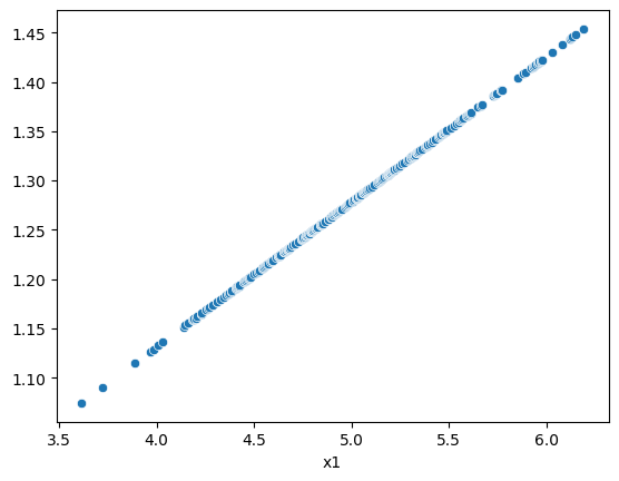
Here, we do not know the weights. To estimate them, we start by running simple OLS to get residuals. Next, we regress root of absolute value of residuals against X and save fitted values. Last, we run a weighted least squares model, using the fitted values as \(\sigma\). Then weights are \(1 / \sigma^2\)
Lots of different methods, see here for more details.
# simple OLS without weights
f = 'y_obs ~ x1'
y, X = patsy.dmatrices(f, df, return_type='dataframe')
mod_ols = sm.OLS(y, X)
res_ols = mod_ols.fit()

# regress root of absolute deviation against X
mod_resid = sm.OLS(np.sqrt(abs(res_ols.resid)), X)
res_resid = mod_resid.fit()
# plot true weights, w against fitted values
sns.scatterplot(w, res_resid.fittedvalues)
/home/chansoo/projects/statsbook/.venv/lib/python3.8/site-packages/seaborn/_decorators.py:36: FutureWarning: Pass the following variables as keyword args: x, y. From version 0.12, the only valid positional argument will be `data`, and passing other arguments without an explicit keyword will result in an error or misinterpretation.
  warnings.warn(
<Axes: xlabel='x1'>
mod_2stage = sm.WLS(y, X, 1 / (res_resid.fittedvalues**2))
print(mod_2stage.fit().summary())
                            WLS Regression Results
==============================================================================
Dep. Variable:                  y_obs   R-squared:                       0.599
Model:                            WLS   Adj. R-squared:                  0.598
Method:                 Least Squares   F-statistic:                     445.0
Date:                Thu, 01 Jun 2023   Prob (F-statistic):           4.57e-61
Time:                        12:46:06   Log-Likelihood:                -700.31
No. Observations:                 300   AIC:                             1405.
Df Residuals:                     298   BIC:                             1412.
Df Model:                           1
Covariance Type:            nonrobust
==============================================================================
                 coef    std err          t      P>|t|      [0.025      0.975]
------------------------------------------------------------------------------
Intercept      1.1803      1.440      0.820      0.413      -1.653       4.014
x1             3.0483      0.145     21.094      0.000       2.764       3.333
==============================================================================
Omnibus:                        2.501   Durbin-Watson:                   2.027
Prob(Omnibus):                  0.286   Jarque-Bera (JB):                2.208
Skew:                          -0.193   Prob(JB):                        0.332
Kurtosis:                       3.165   Cond. No.                         100.
==============================================================================

Notes:
[1] Standard Errors assume that the covariance matrix of the errors is correctly specified.