OLS: Diagnostics#
Ordinary Least Squares / Linear Regression
import numpy as np
import pandas as pd
import statsmodels.api as sm
import statsmodels.stats.api as sms
from statsmodels.compat import lzip
import seaborn as sns
import matplotlib.pyplot as plt
np.random.seed(0)
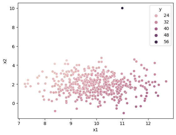
Outliers#
Below uses a fake dataset with one extreme outlier.
n = 500
df = pd.DataFrame({
    "x1":np.random.normal(10,1,n),
    "x2":np.random.normal(2,1,n),
    "e":np.random.normal(0,1,n)
})

df["y"] = 2 + 3*df["x1"] + (-2*df["x2"]) + df["e"]
df.loc[500] = [11, 10, 0, 60]
sns.scatterplot(df["x1"], df["x2"], df['y'])
/home/chansoo/projects/statsbook/.venv/lib/python3.8/site-packages/seaborn/_decorators.py:36: FutureWarning: Pass the following variables as keyword args: x, y, hue. From version 0.12, the only valid positional argument will be `data`, and passing other arguments without an explicit keyword will result in an error or misinterpretation.
  warnings.warn(
<Axes: xlabel='x1', ylabel='x2'>
X = sm.add_constant(df[["x1","x2"]], prepend=False)
mod = sm.OLS(df["y"], X)
res = mod.fit()
print(res.summary())
                            OLS Regression Results
==============================================================================
Dep. Variable:                      y   R-squared:                       0.719
Model:                            OLS   Adj. R-squared:                  0.718
Method:                 Least Squares   F-statistic:                     637.0
Date:                Thu, 01 Jun 2023   Prob (F-statistic):          5.48e-138
Time:                        12:46:00   Log-Likelihood:                -1086.7
No. Observations:                 501   AIC:                             2179.
Df Residuals:                     498   BIC:                             2192.
Df Model:                           2
Covariance Type:            nonrobust
==============================================================================
                 coef    std err          t      P>|t|      [0.025      0.975]
------------------------------------------------------------------------------
x1             3.0629      0.095     32.220      0.000       2.876       3.250
x2            -1.3370      0.091    -14.636      0.000      -1.516      -1.157
const          0.1977      0.974      0.203      0.839      -1.715       2.110
==============================================================================
Omnibus:                      966.837   Durbin-Watson:                   1.318
Prob(Omnibus):                  0.000   Jarque-Bera (JB):          1203045.282
Skew:                          12.899   Prob(JB):                         0.00
Kurtosis:                     241.674   Cond. No.                         106.
==============================================================================

Notes:
[1] Standard Errors assume that the covariance matrix of the errors is correctly specified.
Cook’s Distance:#
where \(y_j{i}\) is the fitted value using the model trained leaving out the i-th observation and p is the # of predictors.
get_influence() and summary_frame prints dfbetas (the difference in each parameter estimatie with and without the
observation). Since the dataset has 501 observations, there are 501 rows in the summary_frame. Note that
this approach may not be ideal if dataset is really big since it runs the model N times
influence = res.get_influence()
df_inf = influence.summary_frame()
df_inf.sort_values('cooks_d', ascending=False)
| dfb_x1 | dfb_x2 | dfb_const | cooks_d | standard_resid | hat_diag | dffits_internal | student_resid | dffits | |
|---|---|---|---|---|---|---|---|---|---|
| 500 | 2.497732 | 16.199589 | -5.195702 | 1.875610e+01 | 19.872939 | 0.124708 | 7.501219 | 43.639717 | 16.472203 |
| 234 | 0.073639 | -0.165384 | -0.048103 | 1.262759e-02 | -1.511125 | 0.016319 | -0.194635 | -1.513080 | -0.194887 |
| 494 | -0.156402 | -0.022125 | 0.150835 | 9.350211e-03 | -1.269424 | 0.017109 | -0.167483 | -1.270205 | -0.167586 |
| 458 | -0.018130 | -0.152639 | 0.039171 | 9.270042e-03 | -1.466662 | 0.012763 | -0.166764 | -1.468363 | -0.166957 |
| 205 | 0.088814 | -0.118305 | -0.070447 | 8.538708e-03 | -1.271721 | 0.015592 | -0.160050 | -1.272511 | -0.160150 |
| ... | ... | ... | ... | ... | ... | ... | ... | ... | ... |
| 62 | 0.000144 | -0.000040 | -0.000150 | 1.864204e-08 | -0.004085 | 0.003340 | -0.000236 | -0.004081 | -0.000236 |
| 264 | 0.000125 | -0.000046 | -0.000120 | 7.438431e-09 | -0.001464 | 0.010298 | -0.000149 | -0.001463 | -0.000149 |
| 322 | -0.000018 | 0.000047 | 0.000002 | 2.188690e-09 | -0.001407 | 0.003305 | -0.000081 | -0.001406 | -0.000081 |
| 296 | -0.000003 | -0.000003 | 0.000001 | 2.518891e-10 | -0.000606 | 0.002055 | -0.000027 | -0.000605 | -0.000027 |
| 472 | 0.000002 | -0.000002 | -0.000002 | 2.455959e-11 | -0.000180 | 0.002257 | -0.000009 | -0.000180 | -0.000009 |
501 rows × 9 columns
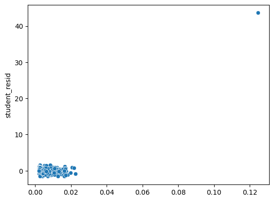
Leverage:#
OLS predicted values are represented as:
Let \(H=X(X'X)^{-1}X'\), then \(\hat{y} = Hy\)
We call “H” the hat matrix. The leverage, \(h_{ii}\) quantifies the influence that the observed response \(y_i\) has on its predicted value \(\hat{y_i}\)
influence = res.get_influence()
# equivalent to "hat_diag" column in df_inf
leverage = influence.hat_matrix_diag
df["leverage"] = leverage
df.sort_values('leverage', ascending=False)
| x1 | x2 | e | y | leverage | |
|---|---|---|---|---|---|
| 500 | 11.000000 | 10.000000 | 0.000000 | 60.000000 | 0.124708 |
| 327 | 12.256723 | 4.225944 | -0.025799 | 30.292483 | 0.022440 |
| 185 | 8.397942 | -0.834555 | -0.177813 | 28.685123 | 0.021730 |
| 89 | 11.054452 | -1.046143 | 0.051820 | 37.307462 | 0.020670 |
| 398 | 11.466579 | 4.594425 | 0.768771 | 27.979658 | 0.019717 |
| ... | ... | ... | ... | ... | ... |
| 267 | 10.088422 | 2.019279 | 2.243602 | 30.470309 | 0.002030 |
| 449 | 9.889611 | 1.883770 | 0.436638 | 28.337930 | 0.002020 |
| 319 | 9.892695 | 2.022960 | -1.297380 | 26.334785 | 0.002019 |
| 302 | 9.881836 | 1.942530 | 0.319432 | 28.079879 | 0.002014 |
| 263 | 9.947433 | 2.024612 | 2.023472 | 29.816546 | 0.002008 |
501 rows × 5 columns
# leverage vs studentized residuals plot
stud_res = res.outlier_test()
sns.scatterplot(leverage, stud_res["student_resid"])
/home/chansoo/projects/statsbook/.venv/lib/python3.8/site-packages/seaborn/_decorators.py:36: FutureWarning: Pass the following variables as keyword args: x, y. From version 0.12, the only valid positional argument will be `data`, and passing other arguments without an explicit keyword will result in an error or misinterpretation.
  warnings.warn(
<Axes: ylabel='student_resid'>
Note the changes in results after outlier removal.
df = df.drop(500)
X = sm.add_constant(df[["x1","x2"]], prepend=False)
mod = sm.OLS(df["y"], X)
res = mod.fit()
print(res.summary())
                            OLS Regression Results
==============================================================================
Dep. Variable:                      y   R-squared:                       0.933
Model:                            OLS   Adj. R-squared:                  0.933
Method:                 Least Squares   F-statistic:                     3480.
Date:                Thu, 01 Jun 2023   Prob (F-statistic):          5.01e-293
Time:                        12:46:00   Log-Likelihood:                -691.18
No. Observations:                 500   AIC:                             1388.
Df Residuals:                     497   BIC:                             1401.
Df Model:                           2
Covariance Type:            nonrobust
==============================================================================
                 coef    std err          t      P>|t|      [0.025      0.975]
------------------------------------------------------------------------------
x1             2.9548      0.043     68.145      0.000       2.870       3.040
x2            -2.0109      0.044    -45.317      0.000      -2.098      -1.924
const          2.5011      0.446      5.602      0.000       1.624       3.378
==============================================================================
Omnibus:                        0.355   Durbin-Watson:                   2.034
Prob(Omnibus):                  0.837   Jarque-Bera (JB):                0.203
Skew:                           0.010   Prob(JB):                        0.903
Kurtosis:                       3.097   Cond. No.                         106.
==============================================================================

Notes:
[1] Standard Errors assume that the covariance matrix of the errors is correctly specified.
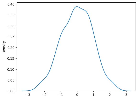
Normality of Residuals#
D’Agostino’s K^2 Test (Omnibus) and Jarque-Bera#
In the bottom section of the OLS summary table below, the Omnibus test and the Jarque-Bera (JB) tests both test the null hypothesis that the residuals are nomrally distributed.
Prob(Omnibus) is 0.205 and Prob(JB) is 0.266 so using both tests, we do not reject the null hypothesis that the residuals are normally distributed.
We plot the density of the residuals to confirm that the residuals appear to be normally distributed.
n = 500
df = pd.DataFrame({
    "x1":np.random.normal(10,1,n),
    "x2":np.random.normal(2,1,n),
    "e":np.random.normal(0,1,n)
})

df["y"] = 2 + 3*df["x1"] + (-2)*df["x2"] + df["e"]

X = sm.add_constant(df[["x1","x2"]], prepend=False)
mod = sm.OLS(df["y"], X)
res = mod.fit()
print(res.summary())
                            OLS Regression Results
==============================================================================
Dep. Variable:                      y   R-squared:                       0.930
Model:                            OLS   Adj. R-squared:                  0.930
Method:                 Least Squares   F-statistic:                     3296.
Date:                Thu, 01 Jun 2023   Prob (F-statistic):          1.45e-287
Time:                        12:46:00   Log-Likelihood:                -678.36
No. Observations:                 500   AIC:                             1363.
Df Residuals:                     497   BIC:                             1375.
Df Model:                           2
Covariance Type:            nonrobust
==============================================================================
                 coef    std err          t      P>|t|      [0.025      0.975]
------------------------------------------------------------------------------
x1             3.0042      0.043     69.126      0.000       2.919       3.090
x2            -1.9924      0.044    -45.698      0.000      -2.078      -1.907
const          1.8701      0.441      4.240      0.000       1.004       2.737
==============================================================================
Omnibus:                        3.168   Durbin-Watson:                   1.801
Prob(Omnibus):                  0.205   Jarque-Bera (JB):                2.645
Skew:                          -0.070   Prob(JB):                        0.266
Kurtosis:                       2.673   Cond. No.                         108.
==============================================================================

Notes:
[1] Standard Errors assume that the covariance matrix of the errors is correctly specified.
sns.kdeplot(res.resid)
<Axes: ylabel='Density'>
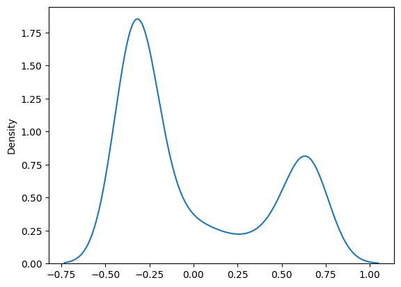
Suppose we generate fake data such that residuals are not normally distributed. The results of the tests and the residual distribution plots change accordingly:
df = pd.DataFrame({
    "x1":np.random.normal(10,1,n),
    "x2":np.random.normal(2,1,n),
    "e":np.random.beta(0.1,0.2,n)
})

df["y"] = 2 + 3*df["x1"] + (-2)*df["x2"] + df["e"]

X = sm.add_constant(df[["x1","x2"]], prepend=False)
mod = sm.OLS(df["y"], X)
res_beta = mod.fit()
print(res_beta.summary())
sns.kdeplot(res_beta.resid)
                            OLS Regression Results
==============================================================================
Dep. Variable:                      y   R-squared:                       0.988
Model:                            OLS   Adj. R-squared:                  0.988
Method:                 Least Squares   F-statistic:                 2.012e+04
Date:                Thu, 01 Jun 2023   Prob (F-statistic):               0.00
Time:                        12:46:00   Log-Likelihood:                -267.08
No. Observations:                 500   AIC:                             540.2
Df Residuals:                     497   BIC:                             552.8
Df Model:                           2
Covariance Type:            nonrobust
==============================================================================
                 coef    std err          t      P>|t|      [0.025      0.975]
------------------------------------------------------------------------------
x1             2.9867      0.018    165.033      0.000       2.951       3.022
x2            -2.0056      0.018   -109.089      0.000      -2.042      -1.969
const          2.4798      0.186     13.333      0.000       2.114       2.845
==============================================================================
Omnibus:                      661.487   Durbin-Watson:                   2.018
Prob(Omnibus):                  0.000   Jarque-Bera (JB):               75.516
Skew:                           0.704   Prob(JB):                     4.00e-17
Kurtosis:                       1.719   Cond. No.                         104.
==============================================================================

Notes:
[1] Standard Errors assume that the covariance matrix of the errors is correctly specified.
<Axes: ylabel='Density'>
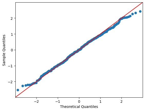
QQ Plots#
A QQ plot sorts your sample in ascending order (here, the sample are the residuals) against the quantiles of a distribution (default is normal distribution).
The number of quantiles is selected to match the size of the sample data.
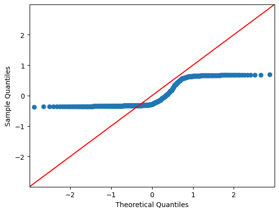
In each of the two plots below, the red line is a 45-degree line. If the distribution is normal, the values should “hug” the line.
g = sm.graphics.qqplot(res.resid, line="45")
g_beta = sm.graphics.qqplot(res_beta.resid, line="45")
Multicollinearity#
Condition number can be used (high numbers indicate multicollinearity), but usually just look at correlation table and plots and VIF
df = pd.DataFrame({
    "x1":np.random.normal(10,1,n),
    "x2":np.random.normal(2,1,n),
    "e":np.random.beta(0.1,0.2,n)
})

df["x3"] = df["x1"] * 1.3 + np.random.normal(0,2,n)
df["x4"] = df["x2"] * 1.3 + np.random.normal(0,1,n)
df["x5"] = df["x1"] * 1.3 + np.random.normal(0,0.5,n)
Condition Number#
# Condition Number
np.linalg.cond(res.model.exog)
108.14224830979715
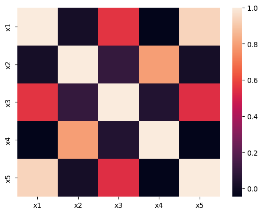
Correlation Matrix#
features = ["x1","x2","x3","x4","x5"]
corr_mat = df[features].corr()
corr_mat
| x1 | x2 | x3 | x4 | x5 | |
|---|---|---|---|---|---|
| x1 | 1.000000 | 0.011713 | 0.555447 | -0.046231 | 0.936899 |
| x2 | 0.011713 | 1.000000 | 0.097119 | 0.794966 | 0.014678 |
| x3 | 0.555447 | 0.097119 | 1.000000 | 0.051660 | 0.540569 |
| x4 | -0.046231 | 0.794966 | 0.051660 | 1.000000 | -0.044700 |
| x5 | 0.936899 | 0.014678 | 0.540569 | -0.044700 | 1.000000 |
sns.heatmap(corr_mat)
<Axes: >
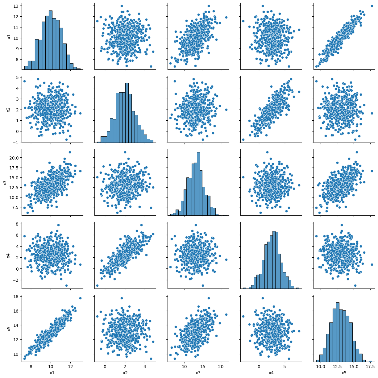
g = sns.PairGrid(df[features])
g.map_diag(sns.histplot)
g.map_offdiag(sns.scatterplot)
<seaborn.axisgrid.PairGrid at 0x7f6b44766970>
VIF#
The variance inflation factor is a measure for the increase of the variance of the parameter estimates if an additional variable, given by exog_idx is added to the linear regression. It is a measure for multicollinearity of the design matrix.
To get VIF, pick each feature and regress it against all other features. For each regression, the factor is calculated as \(VIF = \frac{1}{1-R^2}\)
Generally, VIF > 5 indicates high multicollinearity
from statsmodels.stats.outliers_influence import variance_inflation_factor
X = df[features]
vif_data = pd.DataFrame()
vif_data["feature"] = X.columns
vif_data["VIF"] = [variance_inflation_factor(X.values, i)
                          for i in range(len(X.columns))]
vif_data
| feature | VIF | |
|---|---|---|
| 0 | x1 | 757.478874 |
| 1 | x2 | 14.286991 |
| 2 | x3 | 48.562106 |
| 3 | x4 | 9.554965 |
| 4 | x5 | 734.991722 |
Heteroskedasticity tests#
Also see: Breush-Pagan test and Goldfeld-Quandt test
n = 500
df = pd.DataFrame({
    "x1":np.random.normal(10,1,n),
    "x2":np.random.normal(2,1,n),
    "e":np.random.normal(0,1,n)
})

df["y"] = 2 + 3*df["x1"] + (-2)*df["x2"] + df["e"]

X = sm.add_constant(df[["x1","x2"]], prepend=False)
mod = sm.OLS(df["y"], X)
res = mod.fit()
print(res.summary())
                            OLS Regression Results
==============================================================================
Dep. Variable:                      y   R-squared:                       0.921
Model:                            OLS   Adj. R-squared:                  0.921
Method:                 Least Squares   F-statistic:                     2904.
Date:                Thu, 01 Jun 2023   Prob (F-statistic):          6.61e-275
Time:                        12:46:02   Log-Likelihood:                -715.58
No. Observations:                 500   AIC:                             1437.
Df Residuals:                     497   BIC:                             1450.
Df Model:                           2
Covariance Type:            nonrobust
==============================================================================
                 coef    std err          t      P>|t|      [0.025      0.975]
------------------------------------------------------------------------------
x1             2.9856      0.047     63.018      0.000       2.893       3.079
x2            -2.0059      0.045    -44.356      0.000      -2.095      -1.917
const          2.1361      0.480      4.455      0.000       1.194       3.078
==============================================================================
Omnibus:                        1.417   Durbin-Watson:                   2.108
Prob(Omnibus):                  0.492   Jarque-Bera (JB):                1.355
Skew:                          -0.023   Prob(JB):                        0.508
Kurtosis:                       2.749   Cond. No.                         109.
==============================================================================

Notes:
[1] Standard Errors assume that the covariance matrix of the errors is correctly specified.
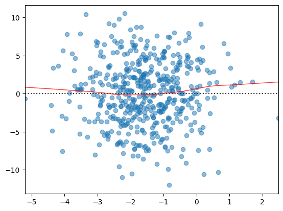
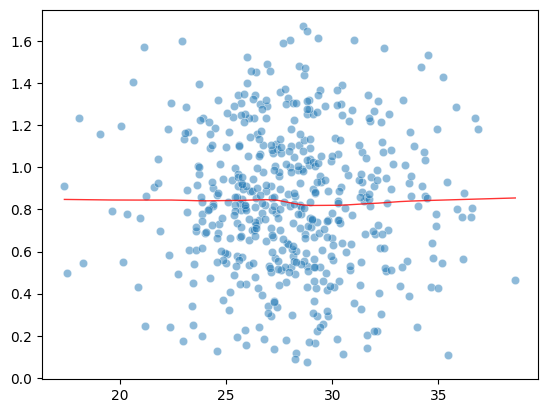
Plot Sqrt(Standarized Residual) vs Fitted values
Horizontal line suggests homoscedasticity
model_norm_residuals = res.get_influence().resid_studentized_internal
model_norm_residuals_abs_sqrt = np.sqrt(np.abs(model_norm_residuals))
sns.scatterplot(res.predict(), model_norm_residuals_abs_sqrt, alpha=0.5)
sns.regplot(res.predict(), model_norm_residuals_abs_sqrt,
            scatter=False,
            ci=False,
            lowess=True,
            line_kws={'color': 'red', 'lw': 1, 'alpha': 0.8})
/home/chansoo/projects/statsbook/.venv/lib/python3.8/site-packages/seaborn/_decorators.py:36: FutureWarning: Pass the following variables as keyword args: x, y. From version 0.12, the only valid positional argument will be `data`, and passing other arguments without an explicit keyword will result in an error or misinterpretation.
  warnings.warn(
<Axes: >
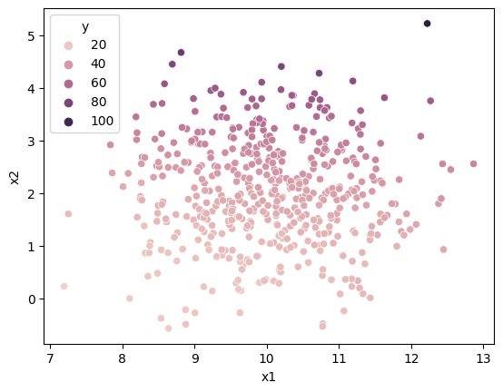
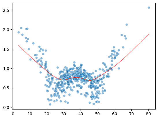
Heteroscedasticity may occur if misspecified model:
n = 500
df = pd.DataFrame({
    "x1":np.random.normal(10,1,n),
    "x2":np.random.normal(2,1,n),
    "e":np.random.normal(0,1,n)
})

df["y"] = 2 + 2*df["x1"] + (3)*df["x2"]**2 + df["e"]

X = sm.add_constant(df[["x1","x2"]], prepend=False)
mod = sm.OLS(df["y"], X)
res = mod.fit()
sns.scatterplot(df["x1"], df["x2"], df["y"])
/home/chansoo/projects/statsbook/.venv/lib/python3.8/site-packages/seaborn/_decorators.py:36: FutureWarning: Pass the following variables as keyword args: x, y, hue. From version 0.12, the only valid positional argument will be `data`, and passing other arguments without an explicit keyword will result in an error or misinterpretation.
  warnings.warn(
<Axes: xlabel='x1', ylabel='x2'>
model_norm_residuals = res.get_influence().resid_studentized_internal
model_norm_residuals_abs_sqrt = np.sqrt(np.abs(model_norm_residuals))
sns.scatterplot(res.predict(), model_norm_residuals_abs_sqrt, alpha=0.5)
sns.regplot(res.predict(), model_norm_residuals_abs_sqrt,
            scatter=False,
            ci=False,
            lowess=True,
            line_kws={'color': 'red', 'lw': 1, 'alpha': 0.8})
/home/chansoo/projects/statsbook/.venv/lib/python3.8/site-packages/seaborn/_decorators.py:36: FutureWarning: Pass the following variables as keyword args: x, y. From version 0.12, the only valid positional argument will be `data`, and passing other arguments without an explicit keyword will result in an error or misinterpretation.
  warnings.warn(
/home/chansoo/projects/statsbook/.venv/lib/python3.8/site-packages/seaborn/_decorators.py:36: FutureWarning: Pass the following variables as keyword args: x, y. From version 0.12, the only valid positional argument will be `data`, and passing other arguments without an explicit keyword will result in an error or misinterpretation.
  warnings.warn(
<Axes: >
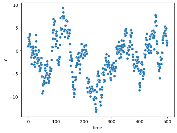
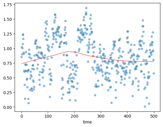
Heteroscedasticity may occur if autocorrelation:
n = 500
df = pd.DataFrame({
    "x1":np.random.normal(0,1,n),
    "time":np.arange(0,n),
    "e":np.random.normal(0,1,n)
})

y_list = [0]
for i in range(n):
    y = df.loc[i,"x1"] + 0.95*y_list[i] + df.loc[i,"e"]
    y_list.append(y)

df["y"] = y_list[1:]

X = sm.add_constant(df[["x1","time"]], prepend=False)
mod = sm.OLS(df["y"], X)
res = mod.fit()
sns.scatterplot(df["time"], df["y"])
/home/chansoo/projects/statsbook/.venv/lib/python3.8/site-packages/seaborn/_decorators.py:36: FutureWarning: Pass the following variables as keyword args: x, y. From version 0.12, the only valid positional argument will be `data`, and passing other arguments without an explicit keyword will result in an error or misinterpretation.
  warnings.warn(
<Axes: xlabel='time', ylabel='y'>
model_norm_residuals = res.get_influence().resid_studentized_internal
model_norm_residuals_abs_sqrt = np.sqrt(np.abs(model_norm_residuals))
sns.scatterplot(df["time"], model_norm_residuals_abs_sqrt, alpha=0.5)
sns.regplot(df["time"], model_norm_residuals_abs_sqrt,
            scatter=False,
            ci=False,
            lowess=True,
            line_kws={'color': 'red', 'lw': 1, 'alpha': 0.8})
/home/chansoo/projects/statsbook/.venv/lib/python3.8/site-packages/seaborn/_decorators.py:36: FutureWarning: Pass the following variables as keyword args: x, y. From version 0.12, the only valid positional argument will be `data`, and passing other arguments without an explicit keyword will result in an error or misinterpretation.
  warnings.warn(
/home/chansoo/projects/statsbook/.venv/lib/python3.8/site-packages/seaborn/_decorators.py:36: FutureWarning: Pass the following variables as keyword args: x, y. From version 0.12, the only valid positional argument will be `data`, and passing other arguments without an explicit keyword will result in an error or misinterpretation.
  warnings.warn(
<Axes: xlabel='time'>
Linearity tests#
Also see Harvey-Collier multiplier test for Null hypothesis that the linear specification is correct.
Plot residuals aggainst fitted values
(or plot observed vs predicted values)
sns.residplot(
    res.predict(),
    res.resid,
    lowess=True,
    scatter_kws={'alpha': 0.5},
    line_kws={'color': 'red', 'lw': 1, 'alpha': 0.8},
)
<Axes: >